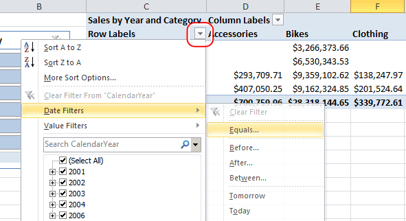
Filter dates in a PivotTable or PivotChart report

The Mark as Date Table dialog box appears when you click Mark as Date Table button or choose Date Table Settings in the Design tab of the Power Pivot window. With the Mark as Date Table dialog box, you specify a unique date column, which enables the use of advanced date filters against Power Pivot data in Excel pivot reports.

Advanced date filters appear for row and column labels in a PivotTable or PivotChart when you add a field from the date table to the Row Labels or Column Labels of the Power Pivot field list.

To change the date properties

1. In the Power Pivot window, select a table that contains dates.

2. In the Design tab, click Mark as Date Table.

3. In the dialog box, select a column that contains unique values, with no blank values.

4. Click OK.

To use advanced date filters

1. Navigate to a PivotTable or PivotChart in the same workbook.

2. Add a column from the Date table to the Column Labels or Row Labels area of the Power Pivot field list.

3. Click the down arrow next to Column Labels or Row Labels in the PivotTable.

4. Point to Date Filters, and then select a filter from the list.

   

Top of Page