When to use Calculated Columns and Calculated Fields

When first learning how to use Power Pivot, most users discover the real power is in aggregating or calculating a result in some way. If your data has a column with numeric values, you can easily aggregate it by selecting it in a PivotTable or Power View Field List. By nature, because it's numeric, it will automatically be summed, averaged, counted, or whatever type of aggregation you select. This is known as an implicit measure. Implicit measures are great for quick and easy aggregation, but they have limits, and those limits can almost always be overcome with explicit measures and calculated columns.

Let's first look at an example where we use a calculated column to add a new text value for each row in a table named Product. Each row in the Product table contains all sorts of information about each product we sell. We have columns for Product Name, Color, Size, Dealer Price, etc.. We have another related table named Product Category that contains a column ProductCategoryName. What we want is for each product in the Product table to include the product category name from the Product Category table. In our Product table, we can create a calculated column named Product Category like this:

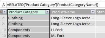
Our new Product Category formula uses the RELATED DAX function to get values from the ProductCategoryName column in the related Product Category table and then enters those values for each product (each row) in the Product table.

This is a great example of how we can use a calculated column to add a fixed value for each row that we can use later in the ROWS, COLUMNS, or FILTERS area of PivotTable or in a Power View report.

Let's create another example where we want to calculate a profit margin for our product categories. This is a common scenario, even in a lot of tutorials. We have a Sales table in our data model that has transaction data, and there is a relationship between the Sales table and the Product Category table. In the Sales table, we have a column that has sales amounts and another column that has costs.

We can create a calculated column that calculates a profit amount for each row by subtracting values in the COGS column from values in the SalesAmount column, like this:

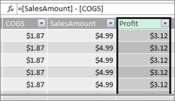
Now, we can create a PivotTable and drag the Product Category field to COLUMNS, and our new Profit field into the VALUES area (a column in a table in PowerPivot is a Field in the PivotTable Field List). The result is an implicit measure named Sum of Profit. It's an aggregated amount of values from the profit column for each of the different product categories. Our result looks like this:

In this case, Profit only makes sense as a field in VALUES. If we were to put Profit in the COLUMNS area, our PivotTable would look like this:

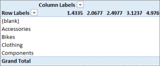
Our Profit field doesn't provide any useful information when it's placed in COLUMNS, ROWS, or FILTERS areas. It only makes sense as an aggregated value in the VALUES area.

What we've done is create a column named Profit that calculates a profit margin for each row in the Sales table. We then added Profit to the VALUES area of our PivotTable, automatically creating an implicit measure, where a result is calculated for each of the product categories. If you're thinking we really calculated profit for our product categories twice, you are correct. We first calculated a profit for each row in the Sales table, and we then added Profit to the VALUES area where it was aggregated for each of the product categories. If you're also thinking we didn't really need to create the Profit calculated column, you are also correct. But, how then do we calculate our profit without creating a Profit calculated column?

Profit, would really be better calculated as an explicit measure.

For now, we're going to leave our Profit calculated column in the Sales table and Product Category in COLUMNS and Profit in VALUES of our PivotTable, to compare our results.

In the calculation area of our Sales table, we're going to create a measure named Total Profit(to avoid naming conflicts). In the end, it will yield the same results as what we did before, but without a Profit calculated column.

First, in the Sales table, we select the SalesAmount column and then click AutoSum to create an explicit Sum of SalesAmountmeasure. Remember, an explicit measure is one we create in the calculation area of a table in Power Pivot. We do the same for the COGS column. We'll rename these Total SalesAmount and Total COGS to make them easier to identify.

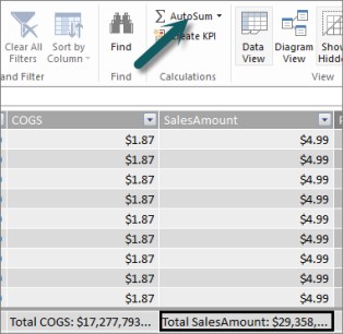
Then we create another measure with this formula:

Total Profit:=[ Total SalesAmount] - [Total COGS]

Note: We could also write our formula as Total Profit:=SUM([SalesAmount]) - SUM([COGS]), but by creating separate Total SalesAmount and Total COGS measures, we can use them in our PivotTable too, and we can use them as arguments in all sorts of other measure formulas.

After changing our new Total Profit measure's format to currency, we can add it to our PivotTable.

You can see our new Total Profit measure returns the same results as creating a Profit calculated column and then placing it in VALUES. The difference is our Total Profit measure is far more efficient and makes our data model cleaner and leaner because we are calculating at the time and only for the fields we select for our PivotTable. We don't really need that Profit calculated column after all.

Why is this last part important? Calculated columns add data to the data model, and data takes up memory. If we refresh the data model, processing resources are also needed to recalculate all of the values in the Profit column. We don't really need to take up resources like this because we really want to calculate our profit when we select the fields we want Profit for in the PivotTable, like product categories, region, or by dates.

Let's look at another example. One where a calculated column creates results that at first glance look correct, but….

In this example, we want to calculate sales amounts as a percentage of total sales. We create a calculated column named % of Sales in our Sales table, like this:

Our formula states: For each row in the Sales table, divide the amount in the SalesAmount column by the SUM total of all amounts in the SalesAmount column.

If we create a PivotTable and add Product Category to COLUMNS and select our new % of Sales column to put it into VALUES, we get a sum total of % of Sales for each of our product categories.

Ok. This looks good so far. But, let's add a slicer. We add Calendar Year and then select a year. In this case, we select 2007. This is what we get.

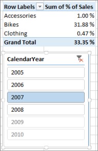
At first glance, this might still appear correct. But, our percentages should really total 100%, because we want to know percentage of total sales for each of our product categories for 2007. So what went wrong?

Our % of Sales column calculated a percent for each row that is the value in the SalesAmount column divided by the sum total of all values in the SalesAmount column. Values in a calculated column are fixed. They are an immutable result for each row in the table. When we added % of Sales to our PivotTable it was aggregated as a sum of all values in the SalesAmount column. That sum of all values in the % of Sales column will always be 100%.

Tip: Be sure to read Context in DAX Formulas. It provides a good understanding of row level context and filter context, which is what we are describing here.

We can delete our % of Sales calculated column because it's not going to help us. Instead, We're going to create a measure that correctly calculates our percent of total sales, regardless of any filters or slicers applied.

Remember the TotalSalesAmount measure we created earlier, the one that simply sums the SalesAmount column? We used it as an argument in our Total Profit measure, and we're going to use it again as an argument in our new calculated field.

Tip: Creating explicit measures like Total SalesAmount and Total COGS are not only useful themselves in a PivotTable or report, but they are also useful as arguments in other measures when you need the result as an argument. This makes your formulas more efficient and easier to read. This is good data modeling practice.

We create a new measure with the following formula:

% of Total Sales:=([Total SalesAmount]) / CALCULATE([Total SalesAmount], ALLSELECTED())

This formula states: Divide the result from Total SalesAmount by the sum total of SalesAmount without any column or row filters other than those defined in the PivotTable.

Tip: Be sure to read about CALCULATE and ALLSELECTED functions in the DAX Reference.

Now, if we add our new % of Total Sales to the PivotTable, we get:

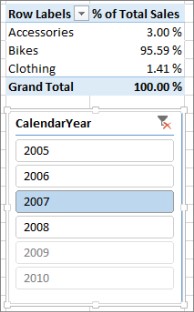
That looks a better. Now our % of Total Sales for each product category is calculated as a percentage of total sales for the 2007 year. If we select a different year, or more than one year in the CalendarYear slicer, we get new percentages for our product categories, but our grand total is still 100%. We can add other slicers and filters too. Our % of Total Sales measure will always produce a percentage of total sales regardless of any slicers or filters applied. With measures, the result is always calculated according to the context determined by the fields in COLUMNS and ROWS, and by any filters or slicers that are applied. This is the power of measures.

Here are a few guidelines to help you when deciding whether or not a calculated column or a measure is right for a particular calculation need:

Use calculated columns

• If you want your new data to appear on ROWS, COLUMNS, or in FILTERS in a PivotTable, or on an AXIS, LEGEND, or, TILE BY in a Power View visualization, you must use a calculated column. Just like regular columns of data, calculated columns can be used as a field in any area, and if they are numeric they can be aggregated in VALUES too.

• If you want your new data to be a fixed value for the row. For example, you have a date table with a column of dates, and you want another column that contains just the number of the month. You can create a calculated column that calculates just the month number from the dates in the Date column. For example, =MONTH('Date'[Date]).

• If you want to add a text value for each row to a table, use a calculated column. Fields with text values can never be aggregated in VALUES. For example, =FORMAT('Date'[Date],"mmmm") gives us the month name for each date in the Date column in the Date table.

Use measures

• If the result of your calculation will always be dependent on the other fields you select in a PivotTable.

• If you need to do more complex calculations, like calculate a count based on a filter of some sort, or calculate a year-over-year, or variance, use a calculated field.

• If you want to keep the size of your workbook to a minimum and maximize its performance, create as many of your calculations as measures as possible. In many cases, all of your calculations can be measures, significantly reducing workbook size and speeding up refresh time.

Keep in-mind, there is nothing wrong with creating calculated columns like we did with our Profit column, and then aggregating it in a PivotTable or report. It's actually a really good and easy way to learn about and create your own calculations. As your understanding of these two extremely powerful features of Power Pivot grows, you will want to create the most efficient and accurate data model you can. Hopefully what you've learned here helps. There are some other really great resources out there that can help you too. Here are just a few: Context in DAX Formulas, Aggregations in Power Pivot, and DAX Resource Center. And, while it's a bit more advanced, and directed towards accounting and finance professionals, the Profit and Loss Data Modeling and Analysis with Microsoft Power Pivot in Excel sample is loaded with great data modeling and formula examples.