How to correct a n a error

The #N/A error generally indicates that a formula can't find what it's been asked to look for.

Top solution

The most common cause of the #N/A error is with XLOOKUP, VLOOKUP, HLOOKUP, LOOKUP, or MATCH functions if a formula can't find a referenced value. For example, your lookup value doesn't exist in the source data.

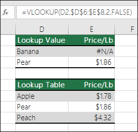
In this case there is no "Banana" listed in the lookup table, so VLOOKUP returns a #N/A error.

Solution: Either make sure that the lookup value exists in the source data, or use an error handler such as IFERROR in the formula. For example, =IFERROR(FORMULA(),0), which says:

• =IF(your formula evaluates to an error, then display 0, otherwise display the formula's result)

You can use "" to display nothing, or substitute your own text: =IFERROR(FORMULA(),"Error Message here")

If you're not sure what to do at this point or what kind of help you need, you can search for similar questions in the Excel Community Forum, or post one of your own.

Note:  Click here if you need help on the #N/A error with a specific function, like VLOOKUP or INDEX/MATCH.

If you want to move forward, then the following checklist provides troubleshooting steps to help you figure out what may have gone wrong in your formulas.

The lookup value and the source data are different data types. For example, you try to have VLOOKUP reference a number, but the source data is stored as text.

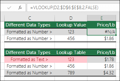
Solution: Ensure that the data types are the same. You can check cell formats by selecting a cell or range of cells, then right-click and select Format Cells > Number (or press Ctrl+1), and change the number format if necessary.

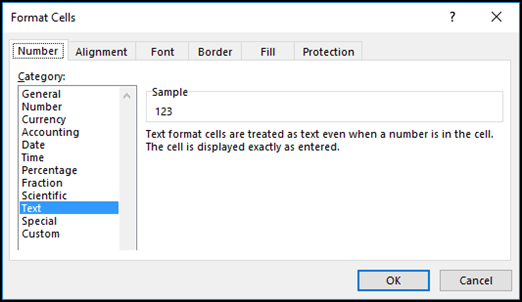
Tip: If you need to force a format change on an entire column, first apply the format you want, then you can use Data > Text to Columns > Finish.

You can use the TRIM function to remove any leading or trailing spaces. The following example uses TRIM nested inside a VLOOKUP function to remove the leading spaces from the names in A2:A7 and return the department name.

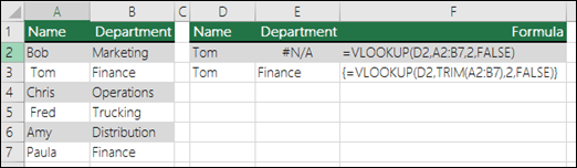
=VLOOKUP(D2,TRIM(A2:B7),2,FALSE)

Note: September 24, 2018 - Dynamic array formulas - If you have a current version of Microsoft 365, and are on the Insiders Fast release channel, then you can input the formula in the top-left-cell of the output range, then press Enter to confirm the formula as a dynamic array formula. Otherwise, the formula must be entered as a legacy array formula by first selecting the output range, input the formula in the top-left-cell of the output range, then press Ctrl+Shift+Enter to confirm it. Excel inserts braces at the beginning and end of the formula for you. For more information on array formulas, see Guidelines and examples of array formulas.

By default, functions that look up information in tables must be sorted in ascending order. However, the VLOOKUP and HLOOKUP worksheet functions contain a range_lookup argument that instructs the function to find an exact match even if the table is not sorted. To find an exact match, set the range_lookup argument to FALSE. Note that using TRUE, which tells the function to look for an approximate match, can not only result in an #N/A error, it can also return erroneous results as seen in the following example.

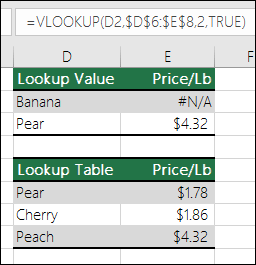
In this example, not only does "Banana" return an #N/A error, "Pear" returns the wrong price. This is caused by using the TRUE argument, which tells the VLOOKUP to look for an approximate match instead of an exact match. There's no close match for "Banana", and "Pear" comes before "Peach" alphabetically. In this case using VLOOKUP with the FALSE argument would return the correct price for "Pear", but "Banana" would still result in a #N/A error, since there is no corresponding "Banana" in the lookup list.

If you are using the MATCH function, try changing the value of the match_type argument to specify the sort order of the table. To find an exact match, set the match_type argument to 0 (zero).

To fix this, make sure that the range referenced by the array formula has the same number of rows and columns as the range of cells in which the array formula was entered, or enter the array formula into fewer or more cells to match the range reference in the formula.

In this example, cell E2 has referenced mismatched ranges:

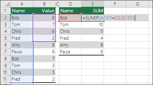
=SUM(IF(A2:A11=D2,B2:B5))

In order for the formula to calculate correctly it needs to be changed so that both ranges reflect rows 2 – 11.

=SUM(IF(A2:A11=D2,B2:B11))

Note: September 24, 2018 - Dynamic array formulas - If you have a current version of Microsoft 365, and are on the Insiders Fast release channel, then you can input the formula in the top-left-cell of the output range, then press Enter to confirm the formula as a dynamic array formula. Otherwise, the formula must be entered as a legacy array formula by first selecting the output range, input the formula in the top-left-cell of the output range, then press Ctrl+Shift+Enter to confirm it. Excel inserts braces at the beginning and end of the formula for you. For more information on array formulas, see Guidelines and examples of array formulas.

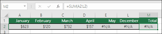
In this case, May-December have #N/A values, so the Total can't calculate and instead returns an #N/A error.

To fix this, check the formula syntax of the function you're using and enter all required arguments in the formula that returns the error. This might require going into the Visual Basic Editor (VBE) to check the function. You can access the VBE from the Developer tab, or with ALT+F11.

To fix this, verify that the workbook that contains the user-defined function is open and that the function is working properly.

To fix this, verify that the arguments in that function are correct and used in the correct position.

To fix this, press Ctrl+Atl+F9 to recalculate the sheet

You can use the Function Wizard to help if you are not sure of the proper arguments. Select the cell with the formula in question, then go to the Formula tab on the Ribbon and press Insert Function.

Excel will automatically load the Wizard for you:

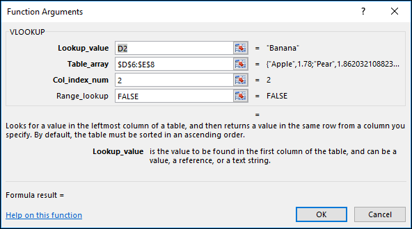
As you click on each argument, Excel will give you the appropriate information for each one.

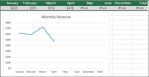
#N/A can be useful! It is a common practice to use #N/A when using data like the following example for charts, as #N/A values won't plot on a chart. Here are examples of what a chart looks like with 0's vs. #N/A.

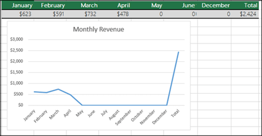
In the previous example, you will see that the 0 values have plotted and are displayed as a flat line on the bottom of the chart, and it then shoots up to display the Total. In the following example you will see the 0 values replaced with #N/A.

For more information on a #NA error appearing in a specific function, see the topics below:

• Correct the #N/A error in VLOOKUP function

• Correct the #N/A error in INDEX/MATCH functions

Top of page

Need more help?

You can always ask an expert in the Excel Tech Community or get support in the Answers community.

See Also

Convert numbers stored as text to numbers

VLOOKUP function

HLOOKUP function

LOOKUP function

MATCH function

Overview of formulas in Excel

How to avoid broken formulas

Detect errors in formulas

Keyboard shortcuts in Excel

All Excel functions (alphabetical)

All Excel functions (by category)