Group or ungroup data in a PivotTable

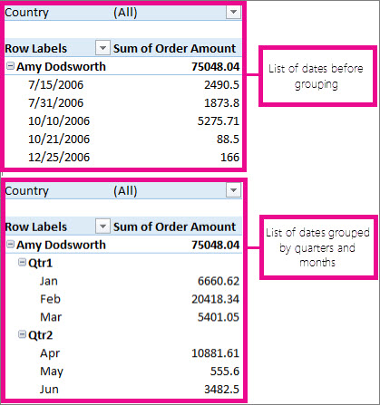
Grouping data in a PivotTable can help you show a subset of data to analyze. For example, you may want to group an unwieldy list of dates or times (date and time fields in the PivotTable) into quarters and months, like this image.

Note: The time grouping feature is new in Excel 2016. With time grouping, relationships across time-related fields are automatically detected and grouped together when you add rows of time fields to your PivotTables. Once grouped together, you can drag the group to your Pivot Table and start your analysis.

Group data

1. In the PivotTable, right-click a value and select Group.

2. In the Grouping box, select Starting at and Ending at checkboxes, and edit the values if needed.

3. Under By, select a time period. For numerical fields, enter a number that specifies the interval for each group.

4. Select OK.

Group selected items

1. Hold Ctrl and select two or more values.

2. Right-click and select Group.

Name a group

1. Select the group.

2. Select Analyze > Field Settings.

3. Change the Custom Name to something you want and select OK.

Ungroup grouped data

1. Right-click any item that is in the group.

2. Select Ungroup.

Need more help?

You can always ask an expert in the Excel Tech Community, get support in the Answers community, or suggest a new feature or improvement on Excel User Voice.

See Also

Create a PivotTable to analyze worksheet data