Outline (group) data in a worksheet
If you have a list of data that you want to group and summarize, you can create an outline of up to eight levels, one for each group. Each inner level, represented by a higher number in the outline symbols, displays detail data for the preceding outer level, represented by a lower number in the outline symbols. Use an outline to quickly display summary rows or columns, or to reveal the detail data for each group. You can create an outline of rows (as shown in the example below), an outline of columns, or an outline of both rows and columns.
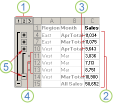 An outlined row of sales data grouped by geographical regions and months with several summary and detail rows displayed. | 1. To display rows for a level, click the appropriate 2. Level 1 contains the total sales for all detail rows. 3. Level 2 contains total sales for each month in each region. 4. Level 3 contains detail rows — in this case, rows 11 through 13. 5. To expand or collapse data in your outline, click the |
What do you want to do?
Create an outline of rows
-
Make sure that each column of the data that you want to outline has a label in the first row, contains similar facts in each column, and that the range has no blank rows or columns.
-
Make sure your detail rows also have a summary row—a subtotal. Do one of the following:
Insert summary rows by using the Subtotal command
-
Use the Subtotal command, which inserts the SUBTOTAL function immediately below or above each group of detail rows and automatically creates the outline for you. For more information about using the Subtotal function, see SUBTOTAL function.
Insert your own summary rows
-
Insert your own summary rows, with formulas, immediately below or above each group of detail rows. For example, under (or above) the rows of sales data for March and April, use the SUM function to subtotal the sales for those months. The table later in this topic shows you an example of this.
-
-
Specify whether the summary rows are located below or above the detail rows. On the Data tab, in the Outline group, click the Outline dialog box launcher.

-
If your summary rows are above your detail rows, clear the Summary rows below detail checkbox. Otherwise, leave the checkbox alone.
-
Outline your data. Do one of the following:
Outline the data automatically
-
If necessary, select a cell in the range of cells you want to outline.
-
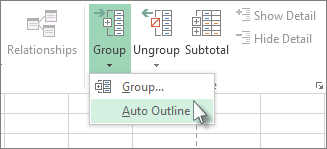
On the Data tab, in the Outline group, click the arrow under Group, and then click Auto Outline.
Outline the data manually
Important: When you manually group outline levels, it's best to have all data displayed to avoid grouping the rows incorrectly.
-
Outline the outer group.
How to outline the outer group
-
Select all of the subordinate summary rows and their related detail rows.
For example, in the data below, row 6 contains the subtotal for rows 2 through 5, and row 10 contains the subtotal for rows 7 through 9, and row 11 contains the grand total. To group all of the detail data for row 11, select rows 2 through 10.
A
B
C
1
Region
Month
Sales
2
East
March
$9,647
3
East
March
$4,101
4
East
March
$7,115
5
East
March
$2,957
6
East
Mar Total
$23,820
7
East
April
$4,257
8
East
April
$1,829
9
East
April
$6,550
10
East
Apr Total
$12,636
11
East Total
$36,456
Important: Do not include the summary row (row 11) in the selection.
-
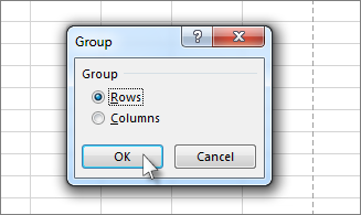
On the Data tab, in the Outline group, click Group, click Rows, and then click OK.
The outline symbols appear beside the group on the screen.
-
-
Optionally, outline an inner, nested group — the detail rows for a given section of your data.
How to outline inner, nested groups (groups of details rows)
-
For each inner, nested group, select the detail rows adjacent to the row that contains the summary row.
In the example below, to group rows 2 through 5, which has a summary row 6, select rows 2 through 5. To group rows 7 through 9, which has a summary row 10, select rows 7 through 9.
A
B
C
1
Region
Month
Sales
2
East
March
$9,647
3
East
March
$4,101
4
East
March
$7,115
5
East
March
$2,957
6
East
Mar Total
$23,820
7
East
April
$4,257
8
East
April
$1,829
9
East
April
$6,550
10
East
Apr Total
$12,636
11
East Total
$36,456
Important: Do not include the summary row in the selection.
-
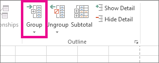
On the Data tab, in the Outline group, click Group.
The outline symbols appear beside the group on the screen.
-
Continue selecting and grouping inner rows until you have created all of the levels that you want in the outline.
-
If you want to ungroup rows, select the rows, and then on the Data tab, in the Outline group, click Ungroup.
You can also ungroup sections of the outline without removing the entire outline. Hold down SHIFT while you click the
 or
or  for the group, and then on the Data tab, in the Outline group, click Ungroup.
Important: If you ungroup an outline while the detail data is hidden, the detail rows may remain hidden. To display the data, drag across the visible row numbers adjacent to the hidden rows. On the Home tab, in the Cells group, click Format, point to Hide & UnHide, and then click Unhide Rows.
-
-
Create an outline of columns
-
Make sure that each row of the data that you want to outline has a label in the first column, contains similar facts in each row, and the range has no blank rows or columns.
-
Insert your own summary columns with formulas immediately to the right or left of each group of detail columns. The table listed in step 4 below shows you an example.
Note: To outline data by columns, you must have summary columns that contain formulas that reference cells in each of the detail columns for that group.
-
Specify whether the location of the summary column is to the right or left of the detail columns. On the Data tab, in the Outline group, click the Outline dialog box launcher.
How to specify the summary column location
-
On the Data tab, in the Outline group, click the Outline dialog box launcher.

-
To specify a summary column to the left of the details column, clear the Summary columns to right of detail check box. To specify a summary column to the right of the details column, select the Summary columns to right of detail check box.
-
Click OK.
-
-
To outline the data, do one of the following:
Outline the data automatically
-
If necessary, select a cell in the range.
-
On the Data tab, in the Outline group, click the arrow below Group and click Auto Outline.
Outline the data manually
Important: When you manually group outline levels, it's best to have all data displayed to avoid grouping columns incorrectly.
-
Outline the outer group.
How to outline the outer group (all the columns except the grand total)
-
Select all of the subordinate summary columns, as well as their related detail data.
In the example below, column E contains the subtotals for columns B through D, and column I contains the subtotals for columns F through H, and column J contains the grand totals. To group all of the detail data for column J, select columns B through I.
A
B
C
D
E
F
G
H
I
J
1
Regn
Jan
Feb
Mar
Q1
Apr
May
Jun
Q2
H1
2
East
371
504
880
1,755
186
653
229
1,068
2,823
3
West
192
185
143
520
773
419
365
1,557
2,077
4
North
447
469
429
1,345
579
180
367
1,126
2,471
5
South
281
511
410
1,202
124
750
200
1,074
2,276
Important: Do not include the summary column J (the grand totals) in the selection.
-
On the Data tab, in the Outline group, click Group.

The outline symbols appear beside the group on the screen.
-
-
Optionally, outline an inner, nested group (individual groups of detail columns).
How to outline the inner, nested group (Groups of detail columns)
-
For each inner, nested group, select the detail columns adjacent to the column that contains the summary column.
In the example below, to group columns B through D, which has a summary column E, select columns B through D. To group columns F through H, which has a summary row I, select columns F through H.
A
B
C
D
E
F
G
H
I
J
1
Regn
Jan
Feb
Mar
Q1
Apr
May
Jun
Q2
H1
2
East
371
504
880
1,755
186
653
229
1,068
2,823
3
West
192
185
143
520
773
419
365
1,557
2,077
4
North
447
469
429
1,345
579
180
367
1,126
2,471
5
South
281
511
410
1,202
124
750
200
1,074
2,276
Important: Do not include the summary column for that group in the selection.
-
On the Data tab, in the Outline group, click Group.

The outline symbols appear beside the group on the screen.
-
-
-
Continue selecting and grouping inner columns until you have created all of the levels that you want in the outline.
-
If you want to ungroup columns, select the columns, and then on the Data tab, in the Outline group, click Ungroup.
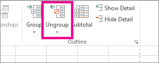
You can also ungroup sections of the outline without removing the entire outline. Hold down SHIFT while you click the  or
or  for the group, and then on the Data tab, in the Outline group, click Ungroup.
If you ungroup an outline while the detail data is hidden, the detail columns may remain hidden. To display the data, drag across the visible column letters adjacent to the hidden columns. On the Home tab, in the Cells group, click Format, point to Hide & Unhide, and then click Unhide Columns
Show or hide outlined data
-
If you don't see the outline symbols
 ,
,  , and
, and  , click the Microsoft Office Button
  and then click Excel Options (Excel 2007), OR, click the File tab (other versions), and then click Options, click the Advanced category, and then under the Display options for this worksheet section, select the worksheet, and then select the Show outline symbols if an outline is applied check box.
 -
Click OK.
-
Do one or more of the following:
Show or hide the detail data for a group
-
To display the detail data within a group, click the
 for the group.
 -
To hide the detail data for a group, click the
 for the group.
Expand or collapse the entire outline to a particular level
-
In the
 outline symbols, click the number of the level that you want. Detail data at lower levels is then hidden.
 For example, if an outline has four levels, you can hide the fourth level while displaying the rest of the levels by clicking
 .
.Show or hide all of the outlined detail data
-
To show all detail data, click the lowest level in the
 outline symbols. For example, if there are three levels, click
  .
. -
To hide all detail data, click
 .
.
-
Customize an outline with styles
For outlined rows, Microsoft Excel uses styles such as RowLevel_1 and RowLevel_2 . For outlined columns, Excel uses styles such as ColLevel_1 and ColLevel_2. These styles use bold, italic, and other text formats to differentiate the summary rows or columns in your data. By changing the way each of these styles is defined, you can apply different text and cell formats to customize the appearance of your outline. You can apply a style to an outline either when you create the outline or after you create it.
Do one or more of the following:
Automatically apply a style to a summary row or column
-
On the Data tab, in the Outline group, click the Outline dialog box launcher.

-
Select the Automatic styles check box.
Apply a style to an existing summary row or column
-
Select the cells that you want to apply outline styles to.
-
On the Data tab, in the Outline group, click the Outline dialog box launcher.

-
Select the Automatic styles check box.
-
Click Apply Styles.
You can also use autoformats to format outlined data.
Copy outlined data
-
If you don't see the outline symbols
 ,
,  , and
, and  , click the Microsoft Office Button
  and then click Excel Options (Excel 2007), OR the File tab (other versions), and then click Options, click the Advanced category, and then under the Display options for this worksheet section, select the worksheet, and then select the Show outline symbols if an outline is applied check box.
 -
Use the outline symbols
 ,
,  , and
, and  to hide the detail data that you don't want copied.
For more information, see the section, Show or hide outlined data.
-
Select the range of summary rows.
-
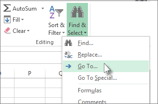
On the Home tab, in the Editing group, click Find & Select, and then click Go To.
-
Click Go To Special.
-
Click Visible cells only.
-
Click OK, and then copy the data.
Hide or remove an outline
Note: No data is deleted when you hide or remove an outline.
Hide an outline
-
(Excel 2007) Click the Microsoft Office Button
 and then click Excel Options OR the File tab (other versions), and then click Options, click the Advanced category, and then under the Display options for this worksheet section, select the worksheet that contains the outline you want to hide and clear the Show outline symbols if an outline is applied check box.
Remove an outline
-
Click the worksheet.
-
One the Data tab, in the Outline group, click Ungroup and click Clear Outline.
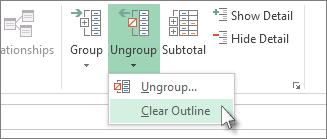
Important: If you remove an outline while the detail data is hidden, the detail rows or columns may remain hidden. To display the data, drag across the visible row numbers or column letters adjacent to the hidden rows and columns. On the Home tab, in the Cells group, click Format, point to Hide & Unhide, and then click Unhide Rows or Unhide Columns.
Create a summary report with a chart
Imagine that you want to create a summary report of your data that only displays totals accompanied by a chart of those totals. In general, you can do the following:
-
Create a summary report.
-
Outline your data.
For more information, see the sections Create an outline of rows or Create an outline of columns.
-
Hide the detail by clicking the outline symbols
 ,
,  , and
, and  to show only the totals as shown in the following example of a row outline:
-
For more information, see the section, Show or hide outlined data.
-
-
Chart the summary report.
-
Select the summary data that you want to chart.
For example, to chart only the Buchanan and Davolio totals, but not the grand totals, select cells A1 through C11 as shown in the above example.
-
Create the chart. For example, on the Insert tab, in the Charts group, click Recommended Charts, or choose another chart type.
For example, if you create the chart by using the Chart Wizard, it would look like the following example.
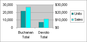
If you show or hide details in the outlined list of data, the chart is also updated to show or hide the data.
-
No comments:
Post a Comment