Dynamically display the contents of a cell or range in a graphic object
To display the contents of a worksheet cell in a shape, text box, or chart element, you can link the shape, text box, or chart element to the cell that contains the data that you want to display. Using the Camera  command, you can also display the contents of a cell range by linking the cell range to a picture.
Because the cell or cell range is linked to the graphic object, changes that you make to the data in that cell or cell range automatically appear in the graphic object.
Dynamically display cell contents in a shape or text box on a worksheet
-
If you do not have an shape or text box in your worksheet, do the following:
-
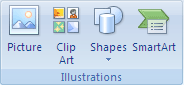
To create an shape, on the Insert tab, in the Illustrations group, click Shapes, and then click the shape that you want to use.
-
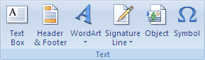
To create a text box, on the Insert tab, in the Text group, click Text Box, and then drag to draw the text box in the text box size that you want.
-
-
On the worksheet, click the shape or text box to which you want to link the cell contents.
-
In the formula bar, type an equal sign (=).
-
Click the worksheet cell that contains the data or text that you want to link to.
Tip: You can also type the reference to the worksheet cell. Include the sheet name, followed by an exclamation point; for example, =Sheet1!F2.
-
Press ENTER.
The contents of the cell is displayed in the shape or text box that you selected.
Note: You cannot use this procedure in a scribble, line, or connector shape.
Dynamically display cell contents in a title, label, or text box on a chart
-
On a chart, click the title, label, or text box that you want to link to a worksheet cell, or do the following to select it from a list of chart elements.
-
Click a chart.
This displays the Chart Tools, adding the Design, Layout, and Format tabs.
-
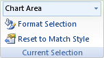
On the Format tab, in the Current Selection group, click the arrow next to the Chart Elements box, and then click the chart element that you want to use.
-
-
In the formula bar, type an equal sign (=).
-
In the worksheet, select the cell that contains the data or text that you want to display in the title, label, or text box on the chart.
Tip: You can also type the reference to the worksheet cell. Include the sheet name, followed by an exclamation point, for example, Sheet1!F2
-
Press ENTER.
The contents of the cell is displayed in the title, label, or text box that you selected.
Dynamically display cell range contents in a picture
-
If you haven't already done so, add Camera
to the Quick Access Toolbar. -
Click the arrow next to the toolbar, and then click More Commands.
-
Under Choose commands from, select All Commands.
-
In the list, select Camera, click Add, and then click OK.
-
-
Select the range of cells.
-
On the Quick Access Toolbar, click Camera
. -
Click a location on a worksheet or chart where you want the picture of the cell range inserted.
The contents of the cell range is displayed in the picture.
-
To format the picture or do other operations, right click the picture and choose a command.
For example, you may want to click the Format Picture command to change the border or make the background transparent.
Need more help?
You can always ask an expert in the Excel Tech Community, get support in the Answers community, or suggest a new feature or improvement on Excel User Voice.
No comments:
Post a Comment