Power Query 101

Note: Power Query is known as Get & Transform in Excel 2016. Information provided here applies to both. To learn more, see Get & Transform in Excel 2016.

Importing data from web page

In this tutorial, you create a query that imports data from a web page. As part of this process, you navigate across tables available on a web page, and apply data transform steps to bring the table into a new shape.

In this article

Task 1: Connect to a web data source

Add a Wikipedia page data source

Task 2: Shape data in the subject table

Step 1: Remove Other Columns to only display columns of interest

Step 2: Replace Values to clean up values in a selected column

Step 3: Filter values in a column

Step 4: Name a query

Step 5: Load the query to a worksheet

Power Query steps created

Task 1: Connect to a web data source

In task 1, you import a Tournament Summary table from the UEFA European Football Championship Wikipedia page at http://en.wikipedia.org/wiki/UEFA_European_Football_Championship.

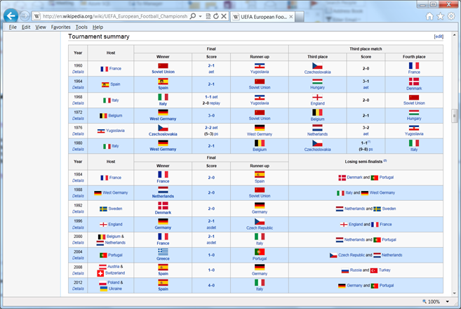
Add a Wikipedia page data source

1. In the POWER QUERY ribbon tab, click From Web.

2. In the Web Content dialog box, in the URL text box, paste the Wikipedia URL (http://en.wikipedia.org/wiki/UEFA_European_Football_Championship).

3. Click OK.

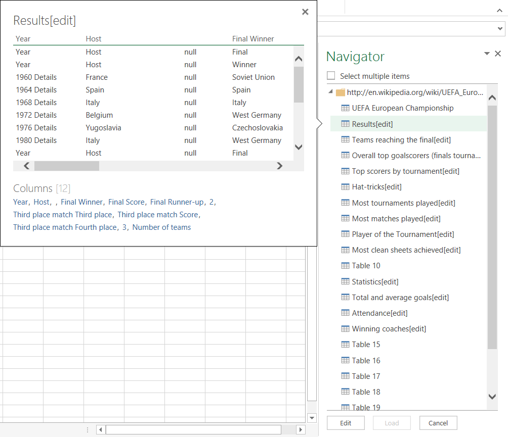
After establishing a connection to the web page, you see a list of tables available on this Wikipedia page in the Navigator pane. You can hover your mouse over each of these tables to preview the data. For each table, you can incrementally apply query activities, such as sort and filter, to shape data. For more information about how to shape data, see Shape data.

In the Navigator pane, double click the Results[edit] table for the Tournament Summary results, or select the Results[edit] table and click Edit Query.

After you open the Query Editor, you can start to shape your query.

Note: For a very quick video on how to display Query Editor, see the end of this article.

Top of Page

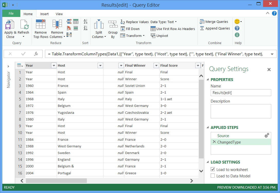
Task 2: Shape data in the subject table

Now that you have the subject table selected for your data query, you learn how to perform various data shaping and cleansing steps.

Step 1: Remove Other Columns to only display columns of interest

In this step, you remove all columns except Year and Final Winners.

1. In the Query Preview grid, select the Year and Final Winners columns (use CTRL + Click).

2. Right-click a column header in the Query Preview grid, and click Remove Other Columns to remove the unselected columns.

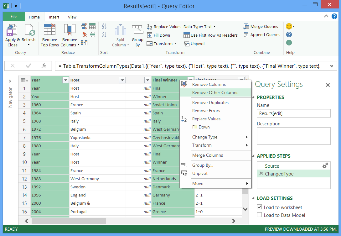
Step 2: Replace Values to clean up values in a selected column

In this step, you replace the Details suffix in the Year column.

1. Select the Year column.

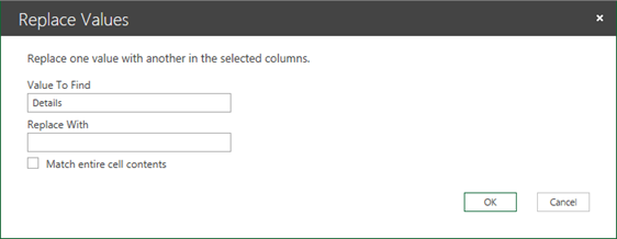
2. In the Query Editor ribbon, click Replace Values or right-click the Year column, and click Replace Values to replace Details with empty text.

3. In the Replace Values dialog box, type Details in the Value to Find text box and leave the Replace With text box empty.

4. Click OK.

   

Step 3: Filter values in a column

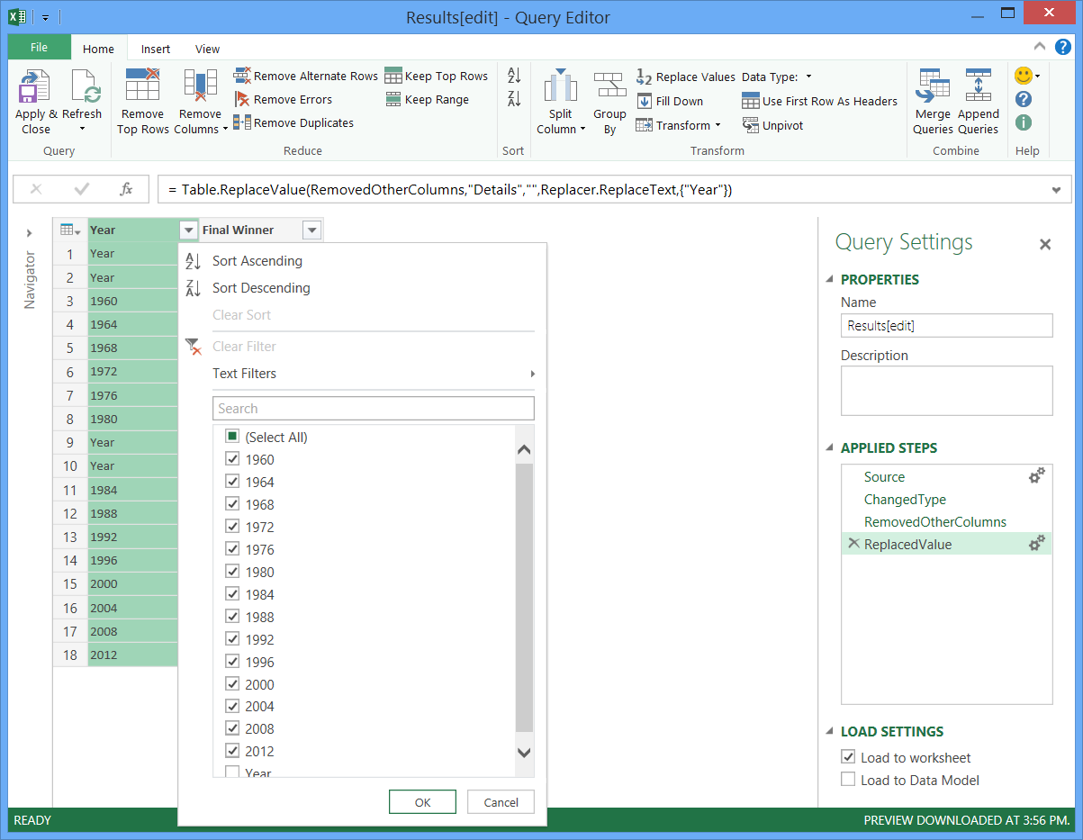
In this step, you filter the Year column to display rows that do not contain "Year".

1. Click the filter drop down arrow on the Year column.

2. In the Filter drop-down, clear the Year option.

3. Click OK.

Step 4: Name a query

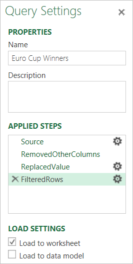
In this step, you name your final query Euro Cup Winners.

1. In the Query Settings pane, in the Name text box, enter Euro Cup Winners. You can also define a query description in the Description text box.

Step 5: Load the query to a worksheet

In this step, you load the Euro Cup Winners query to a worksheet.

1. In the Query Editor ribbon, in the Query group, click Apply & Close.

Power Query steps created

As you perform query activities in Power Query, query steps are created and listed in the Query Settings pane, in the APPLIED STEPS list. Each query step has a corresponding Power Query formula, also known as the "M" language. For more information about the Power Query formula language, see Learn about Power Query formulas.

Task	Query step	Formula
Connect to a web data source	Source	Source{1}[Data]
Remove Other Columns to only display columns of interest	RemovedOtherColumns	Table.SelectColumns (Data1,{"Year", "Final Winner"})
Replace Values to clean up values in a selected column	ReplacedValue	Table.ReplaceValue (RemovedOtherColumns,"Details","" ,Replacer.ReplaceText,{"Year"})
Filter values in a column	FilteredRows	Table.SelectRows (ReplacedValue, each ([Year] <> "Year"))

Top of Page

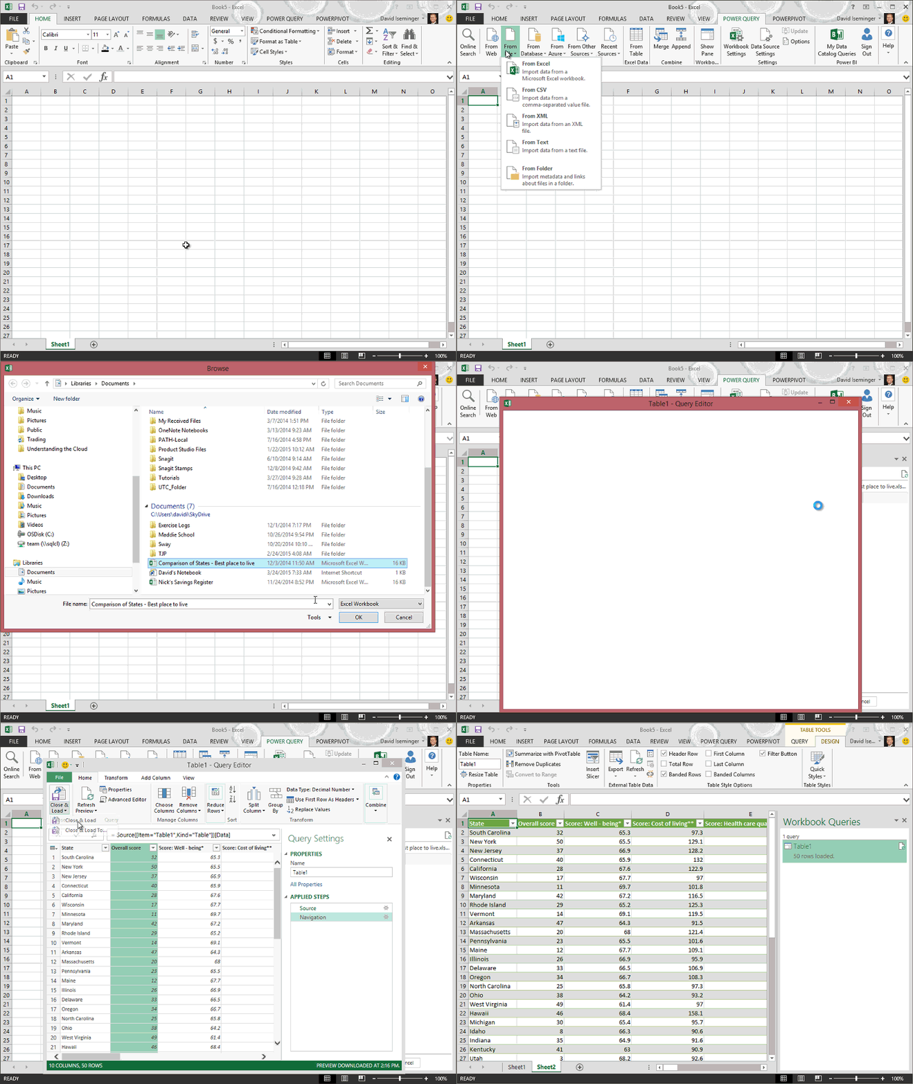
Note: The Query Editor only appears when you load, edit, or create a new query using Power Query. The following video shows the Query Editor window appearing after editing a query from an Excel workbook. To view the Query Editor without loading or editing an existing workbook query, from the Get External Data section in the Power Query ribbon tab, select From Other Sources > Blank Query. The following video shows one way to display the Query Editor.