Microsoft Office Tutorials: Ifs function

Sunday, March 28, 2021

Ifs function

The IFS function checks whether one or more conditions are met, and returns a value that corresponds to the first TRUE condition. IFS can take the place of multiple nested IF statements, and is much easier to read with multiple conditions.

Note: This feature is available on Windows or Mac if you have Office 2019, or if you have a Microsoft 365 subscription. If you are a Microsoft 365 subscriber, make sure you have the latest version of Office.

Simple syntax

Generally, the syntax for the IFS function is:

=IFS([Something is True1, Value if True1,Something is True2,Value if True2,Something is True3,Value if True3)

Please note that the IFS function allows you to test up to 127 different conditions. However, we don't recommend nesting too many conditions with IF or IFS statements. This is because multiple conditions need to be entered in the correct order, and can be very difficult to build, test and update.

Technical details

Syntax

IFS(logical_test1, value_if_true1, [logical_test2, value_if_true2], [logical_test3, value_if_true3],…)

Argument	Description
logical_test1 (required)	Condition that evaluates to TRUE or FALSE.
value_if_true1 (required)	Result to be returned if logical_test1 evaluates to TRUE. Can be empty.
logical_test2…logical_test127 (optional)	Condition that evaluates to TRUE or FALSE.
value_if_true2…value_if_true127 (optional)	Result to be returned if logical_testN evaluates to TRUE. Each value_if_trueN corresponds with a condition logical_testN. Can be empty.

Example 1

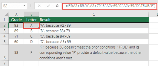
IFS function Grades example. Formula in cell B2 is  =IFS(A2>89,"A",A2>79,"B",A2>69,"C",A2>59,"D",TRUE,"F")

The formula for cells A2:A6 is:

 =IFS(A2>89,"A",A2>79,"B",A2>69,"C",A2>59,"D",TRUE,"F")

Which says IF(A2 is Greater Than 89, then return a "A", IF A2 is Greater Than 79, then return a "B", and so on and for all other values less than 59, return an "F").

Example 2

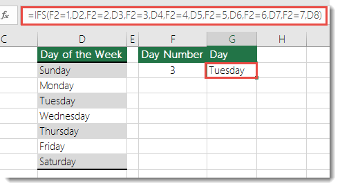
IFS function - Days of the Week example - Formula in cell G2 is  =IFS(F2=1,D2,F2=2,D3,F2=3,D4,F2=4,D5,F2=5,D6,F2=6,D7,F2=7,D8)

The formula in cell G7 is:

 =IFS(F2=1,D2,F2=2,D3,F2=3,D4,F2=4,D5,F2=5,D6,F2=6,D7,F2=7,D8)

Which says IF(the value in cell F2 equals 1, then return the value in cell D2, IF the value in cell F2 equals 2, then return the value in cell D3, and so on, finally ending with the value in cell D8 if none of the other conditions are met).

Remarks

To specify a default result, enter TRUE for your final logical_test argument. If none of the other conditions are met, the corresponding value will be returned. In Example 1, rows 6 and 7 (with the 58 grade) demonstrate this.
 If a logical_test argument is supplied without a corresponding value_if_true, this function shows a "You've entered too few arguments for this function" error message.
 If a logical_test argument is evaluated and resolves to a value other than TRUE or FALSE, this function returns a #VALUE! error.
 If no TRUE conditions are found, this function returns #N/A error.

Need more help?

You can always ask an expert in the Excel Tech Community, get support in the Answers community, or suggest a new feature or improvement on Excel User Voice.

Microsoft Office Tutorials