Unique function

The UNIQUE function returns a list of unique values in a list or range. 

Return unique values from a list of values

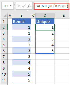
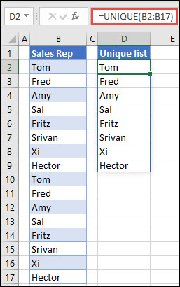
Return unique names from a list of names

Note: This function is currently available only to Microsoft 365 subscribers.

=UNIQUE(array,[by_col],[exactly_once])

The UNIQUE function has the following arguments:

Argument	Description
array Required	The range or array from which to return unique rows or columns
[by_col] Optional	The by_col argument is a logical value indicating how to compare. TRUE will compare columns against each other and return the unique columns FALSE (or omitted) will compare rows against each other and return the unique rows
[exactly_once] Optional	The exactly_once argument is a logical value that will return rows or columns that occur exactly once in the range or array. This is the database concept of unique. TRUE will return all distinct rows or columns that occur exactly once from the range or array FALSE (or omitted) will return all distinct rows or columns from the range or array

Notes: 

• An array can be thought of as a row or column of values, or a combination of rows and columns of values. In the examples above, the arrays for our UNIQUE formulas are range D2:D11, and D2:D17 respectively.

• The UNIQUE function will return an array, which will spill if it's the final result of a formula. This means that Excel will dynamically create the appropriate sized array range when you press ENTER. If your supporting data is in an Excel Table, then the array will automatically resize as you add or remove data from your array range if you're using Structured References. For more details, see this article on Spilled Array Behavior.

• Excel has limited support for dynamic arrays between workbooks, and this scenario is only supported when both workbooks are open. If you close the source workbook, any linked dynamic array formulas will return a #REF! error when they are refreshed.

Examples

Example 1

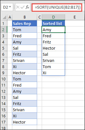
This example uses SORT and UNIQUE together to return a unique list of names in ascending order.

Example 2

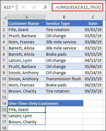
This example has the exactly_once argument set to TRUE, and the function returns only those customers who have had service one time. This can be useful if you want to identify people who have not returned for additional service, so you can contact them.

Example 3

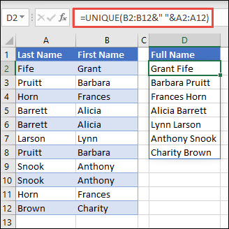
This example uses the ampersand (&) to concatenate last name and first name into a full name. Note that the formula references the entire range of names in A2:A12 and B2:B12. This allows Excel to return an array of all names.

Tips: 

• If you format the range of names as an Excel table, then the formula will automatically update when you add or remove names.

• If you want to sort the list of names, you can add the SORT function: =SORT(UNIQUE(B2:B12&" "&A2:A12))

Example 4

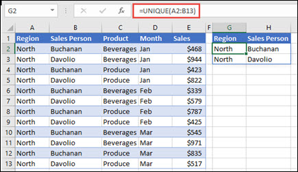
This example compares two columns and returns only the unique values between them.

Need more help?

You can always ask an expert in the Excel Tech Community or get support in the Answers community.

See Also

FILTER function

RANDARRAY function

SEQUENCE function

SORT function

SORTBY function

#SPILL! errors in Excel

Dynamic arrays and spilled array behavior

Implicit intersection operator: @