Create a drop down list

You can help people work more efficiently in worksheets by using drop-down lists in cells. Drop-downs allow people to pick an item from a list that you create.

Want to be walked through this process? Try our new online tutorial for drop-down lists (beta).

Windows macOS Web



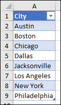
1. In a new worksheet, type the entries you want to appear in your drop-down list. Ideally, you'll have your list items in an Excel table. If you don't, then you can quickly convert your list to a table by selecting any cell in the range, and pressing Ctrl+T.

   

   Notes: 

   • Why should you put your data in a table? When your data is in a table, then as you add or remove items from the list, any drop-downs you based on that table will automatically update. You don't need to do anything else.

   • Now is a good time to Sort data in a range or table in your drop-down list.

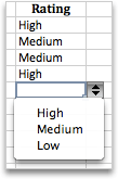
2. Select the cell in the worksheet where you want the drop-down list.

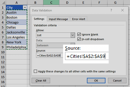
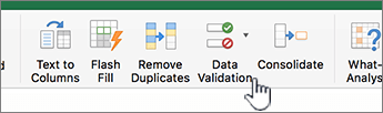
3. Go to the Data tab on the Ribbon, then Data Validation.

   Note: If you can't click Data Validation, the worksheet might be protected or shared. Unlock specific areas of a protected workbook or stop sharing the worksheet, and then try step 3 again.

4. On the Settings tab, in the Allow box, click List.

5. Click in the Source box, then select your list range. We put ours on a sheet called Cities, in range A2:A9. Note that we left out the header row, because we don't want that to be a selection option:

   

6. If it's OK for people to leave the cell empty, check the Ignore blank box.

7. Check the In-cell dropdown box.

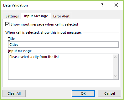
8. Click the Input Message tab.

   • If you want a message to pop up when the cell is clicked, check the Show input message when cell is selected box, and type a title and message in the boxes (up to 225 characters). If you don't want a message to show up, clear the check box.

     

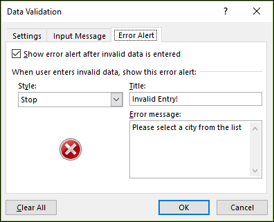
9. Click the Error Alert tab.

   • If you want a message to pop up when someone enters something that's not in your list, check the Show error alert after invalid data is entered box, pick an option from the Style box, and type a title and message. If you don't want a message to show up, clear the check box.

     

10. Not sure which option to pick in the Style box?

    • To show a message that doesn't stop people from entering data that isn't in the drop-down list, click Information or Warning. Information will show a message with this icon and Warning will show a message with this icon .

    • To stop people from entering data that isn't in the drop-down list, click Stop.

      Note: If you don't add a title or text, the title defaults to "Microsoft Excel" and the message to: "The value you entered is not valid. A user has restricted values that can be entered into this cell."

Working with your drop-down list

After you create your drop-down list, make sure it works the way you want. For example, you might want to check to see if Change the column width and row height to show all your entries.

If the list of entries for your drop-down list is on another worksheet and you want to prevent users from seeing it or making changes, consider hiding and protecting that worksheet. For more information about how to protect a worksheet, see Lock cells to protect them.

If you decide you want to change the options in your drop-down list, see Add or remove items from a drop-down list.

To delete a drop-down list, see Remove a drop-down list.

Download our examples

You can download an example workbook with multiple data validation examples like the one in this article. You can follow along, or create your own data validation scenarios. Download Excel data validation examples.

Data entry is quicker and more accurate when you restrict values in a cell to choices from a drop-down list.

Start by making a list of valid entries on a sheet, and sort or rearrange the entries so that they appear in the order you want. Then you can use the entries as the source for your drop-down list of data. If the list is not large, you can easily refer to it and type the entries directly into the data validation tool.

1. Create a list of valid entries for the drop-down list, typed on a sheet in a single column or row without blank cells.

2. Select the cells that you want to restrict data entry in.

3. On the Data tab, under Tools, click Data Validation or Validate.

   

   Note: If the validation command is unavailable, the sheet might be protected or the workbook may be shared. You cannot change data validation settings if your workbook is shared or your sheet is protected. For more information about workbook protection, see Protect a workbook.

4. Click the Settings tab, and then in the Allow pop-up menu, click List.

5. Click in the Source box, and then on your sheet, select your list of valid entries.

   The dialog box minimizes to make the sheet easier to see.

6. Press RETURN or click the Expand   button to restore the dialog box, and then click OK.

   Tips: 

   • You can also type values directly into the Source box, separated by a comma.

   • To modify the list of valid entries, simply change the values in the source list or edit the range in the Source box.

   • You can specify your own error message to respond to invalid data inputs. On the Data tab, click Data Validation or Validate, and then click the Error Alert tab.

See also

Apply data validation to cells

1. In a new worksheet, type the entries you want to appear in your drop-down list. Ideally, you'll have your list items in an Excel table.

   Notes: 

   • Why should you put your data in a table? When your data is in a table, then as you add or remove items from the list, any drop-downs you based on that table will automatically update. You don't need to do anything else.

   • Now is a good time to Sort your data in the order you want it to appear in your drop-down list.

2. Select the cell in the worksheet where you want the drop-down list.

3. Go to the Data tab on the Ribbon, then click Data Validation.

4. On the Settings tab, in the Allow box, click List.

5. If you already made a table with the drop-down entries, click in the Source box, and then click and drag the cells that contain those entries. However, do not include the header cell. Just include the cells that should appear in the drop-down. You can also just type a list of entries in the Source box, separated by a comma like this:

   Fruit,Vegetables,Grains,Dairy,Snacks

6. If it's OK for people to leave the cell empty, check the Ignore blank box.

7. Check the In-cell dropdown box.

8. Click the Input Message tab.

   • If you want a message to pop up when the cell is clicked, check the Show message checkbox, and type a title and message in the boxes (up to 225 characters). If you don't want a message to show up, clear the check box.

9. Click the Error Alert tab.

   • If you want a message to pop up when someone enters something that's not in your list, check the Show Alert checkbox, pick an option in Type, and type a title and message. If you don't want a message to show up, clear the check box.

10. Click OK.

After you create your drop-down list, make sure it works the way you want. For example, you might want to check to see if Change the column width and row height to show all your entries. If you decide you want to change the options in your drop-down list, see Add or remove items from a drop-down list. To delete a drop-down list, see Remove a drop-down list.

Need more help?

You can always ask an expert in the Excel Tech Community or get support in the Answers community.

See also

Apply data validation to cells

All Excel functions (by category)

Creating drop-down lists (free preview)