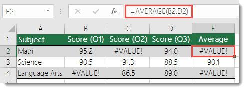
If AVERAGE or SUM refer to cells that contain #VALUE! errors, the formulas will result in a #VALUE! error.

In order to overlook the error values, we'll construct a formula that ignores the errors in the reference range while calculating the average with the remaining "normal" values.
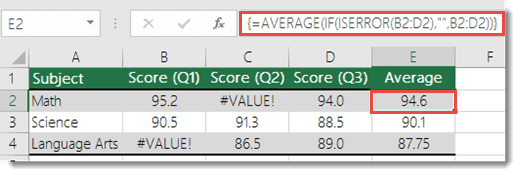
To work around this scenario, we use a combination of AVERAGE along with IF and ISERROR to determine if there is an error in the specified range. This particular scenario requires an array formula:
=AVERAGE(IF(ISERROR(B2:D2),"",B2:D2))
This is an array formula. So you either need to press ENTER (only if you are using Microsoft 365) or CTRL+SHIFT+ENTER in the formula.
Note: If you have a current version of Microsoft 365, then you can simply enter the formula in the output cell, then press ENTER to confirm the formula as a dynamic array formula. Otherwise, the formula must be entered as a legacy array formula by first selecting the output cell, entering the formula in the output cell, and then pressing CTRL+SHIFT+ENTER to confirm it. Excel inserts curly brackets at the beginning and end of the formula for you. For more information on array formulas, see Guidelines and examples of array formulas.

Note: The above function will not only work for #VALUE!, but also for #N/A, #NULL, #DIV/0!, and others.
You could also use SUM in the same fashion:
=SUM(IF(ISERROR(B2:D2),"",B2:D2))
Do you have a specific function question?
Need more help?
You can always ask an expert in the Excel Tech Community or get support in the Answers community.
No comments:
Post a Comment