Convert numbers stored as text to numbers

Numbers that are stored as text can cause unexpected results. Select the cells, and then click to choose a convert option. Or, do the following if that button isn't available.

1. Select a column

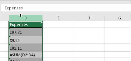
Select a column with this problem. If you don't want to convert the whole column, you can select one or more cells instead. Just be sure the cells you select are in the same column, otherwise this process won't work. (See "Other ways to convert" below if you have this problem in more than one column.)

2. Click this button

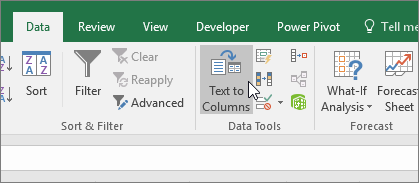
The Text to Columns button is typically used for splitting a column, but it can also be used to convert a single column of text to numbers. On the Data tab, click Text to Columns.

3. Click Apply

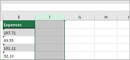
The rest of the Text to Columns wizard steps are best for splitting a column. Since you're just converting text in a column, you can click Apply right away, and Excel will convert the cells.

4. Set the format

Press CTRL + 1 (or + 1 on the Mac). Then select any format.

Note: If you still see formulas that are not showing as numeric results, then you may have Show Formulas turned on. Go to the Formulas tab and make sure Show Formulas is turned off.

Other ways to convert:

Use a formula to convert from text to numbers

You can use the VALUE function to return just the numeric value of the text.

1. Insert a new column

Insert a new column next to the cells with text. In this example, column E contains the text stored as numbers. Column F is the new column.

2. Use the VALUE function

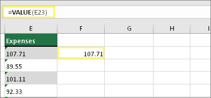
In one of the cells of the new column, type =VALUE() and inside the parentheses, type a cell reference that contains text stored as numbers. In this example it's cell E23.

3. Rest your cursor here

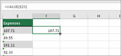
Now you'll fill the cell's formula down, into the other cells. If you've never done this before, here's how to do it: Rest your cursor on the lower-right corner of the cell until it changes to a plus sign.

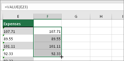
4. Click and drag down

Click and drag down to fill the formula to the other cells. After that's done, you can use this new column, or you can copy and paste these new values to the original column. Here's how to do that: Select the cells with the new formula. Press CTRL + C. Click the first cell of the original column. Then on the Home tab, click the arrow below Paste, and then click Paste Special > Values.

Use Paste Special and Multiply

If the steps above didn't work, you can use this method, which can be used if you're trying to convert more than one column of text.

1. Select a blank cell that doesn't have this problem, type the number 1 into it, and then press Enter.

2. Press CTRL + C to copy the cell.

3. Select the cells that have numbers stored as text.

4. On the Home tab, click Paste > Paste Special.

5. Click Multiply, and then click OK. Excel multiplies each cell by 1, and in doing so, converts the text to numbers.

6. Press CTRL + 1 (or + 1 on the Mac). Then select any format.

Related Topics

Replace a formula with its result
Top ten ways to clean your data
CLEAN function