Change the data series in a chart

After you create your chart, you can change the data series in two ways:

• Use chart filters to show or hide data in your chart.

• Use the Select Data Source box to edit the data in your series or rearrange them on your chart.

Use chart filters

1. Click anywhere in your chart.

2. Click the Chart Filters button next to the chart.

3. On the Values tab, check or uncheck the series or categories you want to show or hide.

   

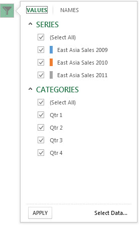
4. Click Apply.

5. If you want to edit or rearrange the data in your series, click Select Data, and then follow steps 2-4 in the next section.

Use the Select Data Source box

1. Right-click your chart, and then pick Select Data.

   You can also get to this box from the Values tab in the Chart Filters gallery.

   

2. In the Legend Entries (Series) box, click the series you want to change.

3. Click Edit, make your changes, and click OK.

   Changes you make may break links to the source data on the worksheet.

4. To rearrange a series, select it, and then click Move Up or Move Down .

Note: You can also add a data series or remove them in this box by clicking the Add or Remove buttons. Removing a data series deletes it from the chart—you can't use chart filters to show it again.

See Also

Rename a data series