Make your Excel spreadsheets accessible

This topic gives you step-by-step instructions to make your Excel spreadsheets accessible to people with disabilities.

People who are blind or have low vision can understand your data more easily if you create your Excel workbooks and charts with accessibility in mind.

Windows Mac iOS Android Online



Windows: Best practices for making Excel spreadsheets accessible

The following table includes key best practices for creating Excel spreadsheets that are accessible to people with disabilities.

What to fix	How to find it	Why fix it	How to fix it
Include alternative text with all visuals and tables. Visual content includes pictures, clip art, SmartArt graphics, shapes, groups, charts, embedded objects, ink, and videos.	To find all instances of missing alternative text in the spreadsheet, use the Accessibility Checker.	Alt text helps people who can't see the screen to understand what's important in images and other visuals. Avoid using text in images as the sole method of conveying important information. If you must use an image with text in it, repeat that text in the document. In alt text, briefly describe the image and mention the existence of the text and its intent.	Add alt text to images Add alt text to SmartArt graphics Add alt text to shapes Add alt text to PivotCharts Add alt text to tables
Add meaningful hyperlink text and ScreenTips.	To determine whether hyperlink text makes sense as standalone information and whether it gives readers accurate information about the destination target, visually scan the workbook.	People who use screen readers sometimes scan a list of links. Links should convey clear and accurate information about the destination. For example, instead of linking to the text Click here, include the full title of the destination page. Tip: You can also add ScreenTips that appear when your cursor hovers over a cell that includes a hyperlink.	Add hyperlink text and ScreenTips
Give all sheet tabs unique names, and remove blank sheets.	To find out whether all sheets that contain content in a workbook have descriptive names and whether there are any blank sheets, use the Accessibility Checker.	Screen readers read sheet names, which provide information about what is found on the worksheet, making it easier to understand the contents of a workbook and to navigate through it.	Rename sheet tabs Delete sheet tabs
Use a simple table structure, and specify column header information.	To ensure that tables don't contain split cells, merged cells, nested tables, or completely blank rows or columns, use the Accessibility Checker.	Screen readers keep track of their location in a table by counting table cells. If a table is nested within another table or if a cell is merged or split, the screen reader loses count and can't provide helpful information about the table after that point. Blank cells in a table could also mislead someone using a screen reader into thinking that there is nothing more in the table. Screen readers also use header information to identify rows and columns.	Add headers to a new table Use headers in an existing table

Add alt text to visuals and tables

The following procedures describe how to add alt text to visuals and tables in your Excel spreadsheets.

Note: We recommend only putting text in the description field and leaving the title blank. This will provide the best experience with most major screen readers including Narrator. For audio and video content, in addition to alt text, include closed captioning for people who are deaf or have limited hearing.

Add alt text to images

Add alt text to images, such as pictures, clip art, and screenshots, so that screen readers can read the text to describe the image to users who can't see the image.

1. Right-click an image.

2. Select Format Picture > Size & Properties.

3. Select Alt Text.

4. Type a description and a title.

   Tip: Include the most important information in the first line, and be as concise as possible.

Add alt text to SmartArt graphics

1. Right-click a SmartArt graphic.

2. Select Format Shape > Shape Options > Size & Properties.

3. Select Alt Text.

4. Type a description and a title.

   Tip: Include the most important information in the first line, and be as concise as possible.

Add alt text to shapes

Add alt text to shapes, including shapes within a SmartArt graphic.

1. Right-click a shape.

2. Select Format Shape > Shape Options > Size & Properties.

3. Select Alt Text.

4. Type a description and a title.

   Tip: Include the most important information in the first line, and be as concise as possible.

Add alt text to PivotCharts

1. Right-click a PivotChart.

2. Select Format Chart Area > Chart Options > Size & Properties.

3. Select Alt Text.

4. Type a description and a title.

   Tip: Include the most important information in the first line, and be as concise as possible.

Add alt text to tables

1. Right-click a table.

2. Select Table > Alternative Text.

3. Type a description and a title.

   Tip: Include the most important information in the first line, and be as concise as possible.

Make hyperlinks, tables, and sheet tabs accessible

The following procedures describe how to make the hyperlinks, tables, and sheet tabs in Excel spreadsheets accessible.

Add hyperlink text and ScreenTips

1. Right-click a cell.

2. Select Hyperlink.

3. In the Text to display box, type the hyperlink text.

4. In the Address box, enter the destination address for the hyperlink.

5. Select the ScreenTip button and, in the ScreenTip text box, type a ScreenTip.

Tip: If the title on the hyperlink's destination page gives an accurate summary of what's on the page, use it for the hyperlink text. For example, this hyperlink text matches the title on the destination page: Templates and Themes for Office Online.

Use headers in an existing table

Specify a header row in a block of cells marked as a table.

1. Position the cursor anywhere in a table.

2. On the Table Tools Design tab, in the Table Style Options group, select the Header Row check box.

3. Type column headings.

Add headers to a new table

Specify a header row in a new block of cells you are marking as a table.

1. Select the cells you want to include in the table.

2. On the Insert tab, in the Tables group, select Table.

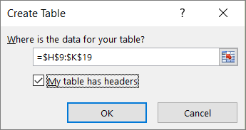
3. Select the My table has headers check box.

4. Select OK.
   Excel creates a header row with the default names Column1, Column2, and so on

5. Type new, descriptive names for each column in the table.

Rename sheet tabs

1. Right-click a sheet tab, and select Rename.

2. Type a brief, unique name for the sheet.

Delete sheet tabs

1. Right-click a sheet tab.

2. Select Delete.

Learn more

• Use Accessibility Checker rules to help ensure your Office documents, spreadsheets, and presentations are accessible

• Make your Word documents accessible

• Make your PowerPoint presentations accessible

• Make your Outlook email accessible

Mac: Best practices for making Excel spreadsheets accessible

The following table includes key best practices for creating Excel spreadsheets that are accessible to people with disabilities.

What to fix	How to find it	Why fix it	How to fix it
Include alternative text with all visuals and tables. Visual content includes pictures, clip art, SmartArt graphics, shapes, groups, charts, embedded objects, ink, and videos.	To find all instances of missing alternative text in the spreadsheet, use the Accessibility Checker.	Alt text helps people who can't see the screen to understand what's important in images and other visuals. Avoid using text in images as the sole method of conveying important information. If you must use an image with text in it, repeat that text in the document. In alt text, briefly describe the image and mention the existence of the text and its intent.	Add alt text to images Add alt text to SmartArt graphics Add alt text to shapes Add alt text to PivotCharts Add alt text to tables
Add meaningful hyperlink text and ScreenTips.	To determine whether hyperlink text makes sense as standalone information and whether it gives readers accurate information about the destination target, visually scan the sheets in your workbook.	People who use screen readers sometimes scan a list of links. Links should convey clear and accurate information about the destination. For example, instead of linking to the text Click here, include the full title of the destination page. Tip: You can also add ScreenTips that appear when your cursor hovers over a cell that includes a hyperlink.	Add hyperlink text and ScreenTips
Give all sheet tabs unique names, and remove blank sheets.	To find out whether all sheets that contain content in a workbook have descriptive names and whether there are any blank sheets, use the Accessibility Checker.	Screen readers read sheet names, which provide information about what is found on the worksheet, making it easier to understand the contents of a workbook and to navigate through it.	Rename sheet tabs Delete a sheet tab
Use a simple table structure, and specify column header information.	To ensure that tables don't contain split cells, merged cells, nested tables, or completely blank rows or columns, use the Accessibility Checker.	Screen readers keep track of their location in a table by counting table cells. If a table is nested within another table or if a cell is merged or split, the screen reader loses count and can't provide helpful information about the table after that point. Blank cells in a table could also mislead someone using a screen reader into thinking that there is nothing more in the table. Screen readers also use header information to identify rows and columns.	Add headers to a new table Use headers in an existing table

Add alt text to visuals and tables

The following procedures describe how to add alt text to visuals and tables in your Excel spreadsheets.

Note:  For audio and video content, in addition to alt text, include closed captioning for people who are deaf or have limited hearing.

Add alt text to images

Add alt text to images, such as pictures, clip art, and screenshots, so that screen readers can read the text to describe the image to users who can't see the image.

1. Right-click an image.

2. Select Format Picture > Size & Properties.

3. Select Alt Text.

4. Type a description and a title.

   Tip: Include the most important information in the first line, and be as concise as possible.

Add alt text to SmartArt graphics

1. Right-click a SmartArt graphic.

2. Select Format Shape > Shape Options > Size & Properties.

3. Select Alt Text.

4. Type a description and a title.

   Tip: Include the most important information in the first line, and be as concise as possible.

Add alt text to shapes

Add alt text to shapes, including shapes within a SmartArt graphic.

1. Right-click a shape.

2. Select Format Shape > Shape Options > Size & Properties.

3. Select Alt Text.

4. Type a description and a title.

   Tip: Include the most important information in the first line, and be as concise as possible.

Add alt text to PivotCharts

1. Right-click a PivotChart.

2. Select Format Chart Area > Chart Options > Size & Properties.

3. Select Alt Text.

4. Type a description and a title.

   Tip: Include the most important information in the first line, and be as concise as possible.

Add alt text to tables

1. Right-click a table.

2. Select Table > Alternative Text.

3. Type a description and a title.

   Tip: Include the most important information in the first line, and be as concise as possible.

Make hyperlinks, tables, and sheet tabs accessible

The following procedures describe how to make the hyperlinks, tables, and sheet tabs in Excel spreadsheets accessible.

Add hyperlink text and ScreenTips

1. Right-click a cell.

2. Select Hyperlink.

3. In the Text to display box, type the hyperlink text.

4. In the Address box, type the destination URL.

5. Select the ScreenTip button and, in the ScreenTip text box, type a ScreenTip.

Tip: If the title on the hyperlink's destination page gives an accurate summary of what's on the page, use it for the hyperlink text. For example, this hyperlink text matches the title on the destination page: Templates and Themes for Office Online.

Use headers in an existing table

Specify a header row in a block of cells marked as a table.

1. Position the cursor anywhere in a table.

2. On the Table tab, select the Header Row check box.

3. Type column headings.

Add headers to a new table

Specify a header row in a new block of cells you are marking as a table.

1. Select the cells you want to include in the table.

2. On the Insert tab, select Table.

3. Select the My table has headers check box.

4. Select OK.
   Excel creates a header row with the default names Column1, Column2, and so on.

5. Type new, descriptive names for each column in the table.

Rename sheet tabs

1. Right-click a sheet tab, and select Rename.

2. Type a brief, unique name for the sheet.

Delete a sheet tab

1. Right-click a sheet tab.

2. Select Delete.

Learn more

• Use Accessibility Checker rules to help ensure your Office documents, spreadsheets, and presentations are accessible

• Make your Word documents accessible

• Make your PowerPoint presentations accessible

• Make your Outlook email accessible

iOS: Best practices for making Excel spreadsheets accessible

The following table includes key best practices for creating Excel spreadsheets that are accessible to people with disabilities.

What to fix	Why fix it	How to fix it
Give all sheet tabs unique names.	Screen readers read sheet names, which provide information about what is found on the worksheet, making it easier to understand the contents of a workbook and to navigate through it.	Rename sheet tabs
Use a simple table structure, and specify column header information.	Screen readers keep track of their location in a table by counting table cells. If a table is nested within another table or if a cell is merged or split, the screen reader loses count and can't provide helpful information about the table after that point. Blank cells in a table could also mislead someone using a screen reader into thinking that there is nothing more in the table. Screen readers also use header information to identify rows and columns.	Use headers in existing tables

Make tables and sheet tabs accessible

The following procedures describe how to make the tables and sheet tabs in your Excel spreadsheets accessible.

Use headers in existing tables

Specify a header row in a block of cells marked as a table.

1. Position the cursor anywhere in a table.

2. To open the Table tab, at the bottom of the screen, at the end of the toolbar, tap the More icon.

3. To select the Header Row option, tap it.

4. In your table, type column headings.

Rename sheet tabs

1. Double-tap a sheet tab.

2. To replace the selected sheet name, type a brief, unique name for the sheet.

Learn more

• Use Accessibility Checker rules to help ensure your Office documents, spreadsheets, and presentations are accessible

• Make your Word documents accessible

• Make your PowerPoint presentations accessible

• Make your Outlook email accessible

Android: Best practices for making Excel spreadsheets accessible

The following table includes key best practices for creating Excel spreadsheets that are accessible to people with disabilities.

What to fix	Why fix it	How to fix it
Include alternative text with all visuals and tables. Visual content includes pictures, clip art, SmartArt graphics, shapes, groups, charts, embedded objects, ink, and videos.	Alt text helps people who can't see the screen to understand what's important in images and other visuals. Avoid using text in images as the sole method of conveying important information. If you must use an image with text in it, repeat that text in the document. In alt text, briefly describe the image and mention the existence of the text and its intent.	Add alt text to images Add alt text to shapes Add alt text to charts
Give all sheet tabs unique names.	Screen readers read sheet names, which provide information about what is found on the worksheet, making it easier to understand the contents of a workbook and to navigate through it.	Rename sheet tabs
Use a simple table structure, and specify column header information.	Screen readers keep track of their location in a table by counting table cells. If a table is nested within another table or if a cell is merged or split, the screen reader loses count and can't provide helpful information about the table after that point. Blank cells in a table could also mislead someone using a screen reader into thinking that there is nothing more in the table. Screen readers also use header information to identify rows and columns.	Add headers to new tables Use headers in existing tables

Add alt text to visuals

The following procedures describe how to add alt text to visuals in your Excel spreadsheets.

Note:  For audio and video content, in addition to alt text, include closed captioning for people who are deaf or have limited hearing.

Add alt text to images

Add alt text to images such as pictures, clip art, and screenshots so that screen readers can read the text to describe the image to users who can't see the image.

1. Select an image.

2. To open the Picture tab, at the bottom of the screen, at the end of the toolbar, tap the up arrow.

3. Scroll down to the Alt Text command, and then tap it.

4. Type a description and a title. Your changes are automatically saved.

   Tip: Include the most important information in the first line, and be as concise as possible.

Add alt text to shapes

Add alt text to shapes including shapes within a SmartArt graphic.

1. Select a shape.

2. To open the Shape tab, at the bottom of the screen, at the end of the toolbar, tap the up arrow.

3. Scroll down to the Alt Text command, and then tap it.

4. Type a description and a title. Your changes are automatically saved.

   Tip: Include the most important information in the first line, and be as concise as possible.

Add alt text to charts

1. Select a chart.

2. To open the Chart tab, at the bottom of the screen, at the end of the toolbar, tap the up arrow.

3. Scroll down to the Alt Text command, and then tap it.

4. Type a description and a title. Your changes are automatically saved.

   Tip: Include the most important information in the first line, and be as concise as possible.

Make tables and sheet tabs accessible

The following procedures describe how to make the tables and sheet tabs in your Excel spreadsheets accessible.

Use headers in existing tables

Specify a header row in a block of cells marked as a table.

1. Position the cursor anywhere in a table.

2. To open the Table tab, at the bottom of the screen, at the end of the toolbar, tap the down arrow.

3. To select the Header Row option, tap it.

   Tip: When the option is selected, it's gray.

4. In your table, type column headings.

Add headers to new tables

Specify a header row in a new block of cells you are marking as a table.

1. Highlight the cells you want to include in the table.

2. To open the Home tab, at the bottom of the screen, at the end of the toolbar, tap the up arrow.

3. Tap Home > Insert.

4. Tap the Table command.

5. Select the Table has headers check box.

Rename sheet tabs

1. Tap and hold a sheet tab, and select Rename.

2. Type a brief, unique name for the sheet.

Learn more

• Use Accessibility Checker rules to help ensure your Office documents, spreadsheets, and presentations are accessible

• Make your Word documents accessible

• Make your PowerPoint presentations accessible

• Make your Outlook email accessible

Office Online: Best practices for making Excel Online spreadsheets accessible

The following table includes key best practices for creating Excel Online spreadsheets that are accessible to people with disabilities.

What to fix	How to find it	Why fix it	How to fix it
Include alternative text with all visuals and tables.	Use the Accessibility Checker in Excel Online to find instances of missing alternative text in the spreadsheet.	Alt text helps people who can't see the screen to understand what's important in tables. Avoid using text in tables as the sole method of conveying important information. In alt text, briefly describe the contents of the table and its intent.	Add alt text to images Add alt text to charts
Add meaningful hyperlink text.	To determine whether hyperlink text makes sense as standalone information and whether it gives readers accurate information about the destination target, visually scan the workbook.	People who use screen readers sometimes scan a list of links. Links should convey clear and accurate information about the destination. For example, instead of linking to the text Click here, include the full title of the destination page.	Add hyperlink text
Give all sheet tabs unique names, and remove blank sheets.	Read the names of the sheet tabs in your workbook, and verify that each sheet has content.	Screen readers read sheet names, which provide information about what is found on the worksheet, making it easier to understand the contents of a workbook and to navigate through it.	Give the workbook a meaningful name Rename sheet tabs Delete sheet tabs
Use a simple table structure, and specify column header information.	Use the Accessibility Checker in Excel Online to ensure that tables don't contain split cells, merged cells, nested tables, or completely blank rows or columns.	Screen readers keep track of their location in a table by counting table cells. If a table is nested within another table or if a cell is merged or split, the screen reader loses count and can't provide helpful information about the table after that point. Blank rows and columns in a table could also mislead someone using a screen reader into thinking that there is nothing more in the table. Screen readers also use header information to identify rows and columns.	Use headers in a table

Add alt text to images and charts

The following procedures describe how to add alt text to images and charts in your Excel Online spreadsheets. To add alt text to tables, use a desktop version of Excel.

Note: We recommend only putting text in the description field and leaving the title blank. This will provide the best experience with most major screen readers including Narrator.

Add alt text to images

1. Right-click the image, and then select Alt Text to open the Alternative Text dialog box.

2. Revise the text in the Description text box.

3. Select OK.

Add alt text to charts

1. Right-click the chart, and then select Alt Text to open the Alternative Text dialog box.

2. Add text in the Description text box.

3. Select OK.

Make hyperlinks, tables, and sheet tabs accessible

The following procedures describe how to make the hyperlinks, tables, and sheet tabs in Excel Online spreadsheets accessible.

Add hyperlink text

1. Right-click a cell.

2. Select Hyperlink.

3. In Display Text, type the text that people will click on. Then, depending on the type of link you want to use, do one of the following:

   • In URL, type or paste the address.

   • In Place in this document, type the location of the cell you want to link to. For example, A6.

   • In Email address, type the email address in the format of someone@example.com.

4. Click OK.

Tip: If the title on the hyperlink's destination page gives an accurate summary of what's on the page, use it for the hyperlink text. For example, this hyperlink text matches the title on the destination page: Templates and Themes for Office Online.

Use headers in a table

1. Select the cells you want to include in the table.

2. On the Insert tab, in the Tables group, select Table.

3. Select the My table has headers check box.

4. Select OK.
   Excel Online creates a header row with the default names Column1, Column2, and so on.

5. Type new, descriptive names for each column in the table.

Note: Use these same steps to add a header to cells in an existing table.

Give the workbook a meaningful name

1. Select File > Save As.

2. Select Save As, and then type a name for the file. Create a name that provides a hint about what kind of data the file contains. If possible, include the date as part of the name.

3. (Optional) Select the Replace existing file check box.

4. Select OK.

Note: If you want to rename a file, select Rename, type the name for the file, and select OK.

Rename sheet tabs

1. Right-click a sheet tab, and select Rename.

2. Type a brief, unique name for the tab that's descriptive of its contents.

3. Select OK.

Delete sheet tabs

1. Right-click a sheet tab.

2. Select Delete.

3. Select OK.

Use the Accessibility Checker in Excel Online

1. Select the Review tab.

2. Select Accessibility Checker.

3. Review the results in the Accessibility Checker. Results are categorized based on the severity of the issue found, as follows:

   • Errors. Includes content that is very difficult or impossible for people with disabilities to understand.

   • Warnings. The content is challenging for people with disabilities to understand.

   • Tips. Tips let you know that, even though people with disabilities can understand the content, it could be better organized or presented to improve their experience.

4. Fix the issues.

Note: The Accessibility Checker inspects your document for all issues that can be fixed in the browser. For a complete inspection, open your document in the desktop app and use the desktop accessibility checker for Windows or Mac.

Learn more

• Use Accessibility Checker rules to help ensure your Office documents, spreadsheets, and presentations are accessible

• Make your Word documents accessible

• Make your PowerPoint presentations accessible

• Make your Outlook email accessible

Technical support for customers with disabilities

Microsoft wants to provide the best possible experience for all our customers. If you have a disability or questions related to accessibility, please contact the Microsoft Disability Answer Desk for technical assistance. The Disability Answer Desk support team is trained in using many popular assistive technologies and can offer assistance in English, Spanish, French, and American Sign Language. Please go to the Microsoft Disability Answer Desk site to find out the contact details for your region.

If you are a government, commercial, or enterprise user, please contact the enterprise Disability Answer Desk.