Display numbers as percentages

This article explains how to display numbers as percentages in Excel 2007. However, it doesn't cover techniques for calculating percentages. To learn how to calculate values, such as sales tax for a certain amount or a percent change in sales between two fiscal quarters, see Calculate percentages.

How Excel 2007 handles percentages

Although formatting numbers as percentages is straightforward, the results you get after applying the format may vary, depending on whether the numbers already exist in your workbook.

Formatting cells that contain numbers If you apply the Percentage format to existing numbers in a workbook, Excel multiplies those numbers by 100 to convert them to percentages. For example, if a cell contains the number 10, Excel multiplies that number by 100, which means that you will see 1000.00% after you apply the Percentage format. This may not be what you expected. To accurately display percentages, before you format the numbers as a percentage, make sure that they have been calculated as percentages, and that they are displayed in decimal format. Percentages are calculated by using the equation amount / total = percentage. For example, if a cell contains the formula =10/100, the result of that calculation is 0.1. If you then format 0.1 as a percentage, the number will be correctly displayed as 10%. To learn more about calculating percentages, see Calculate percentages.
Formatting empty cells Numbers that you type into cells after you apply the Percentage format to those cells are treated differently. Numbers equal to and larger than 1 are converted to percentages by default; and numbers smaller than 1 are multiplied by 100 to convert them to percentages. For example, typing 10 or 0.1 both result in 10.00%. (If you don't want to display the two zeros after the decimal point, it's easy to get rid of them, as explained in the following procedure.)

Top of Page

Display numbers as percentages

To quickly apply percentage formatting to selected cells, click Percent Style Button image in the Number group on the Home tab, or press CTRL+SHIFT+%. If you want more control over the format, or you want to change other aspects of formatting for your selection, you can use the following procedure.

Select the cells that you want to format.

How to select cells, ranges, rows, or columns

To select	Do this
A single cell	Click the cell, or press the arrow keys to move to the cell.
A range of cells	Click the first cell in the range, and then drag to the last cell, or hold down SHIFT while you press the arrow keys to extend the selection. You can also select the first cell in the range, and then press F8 to extend the selection by using the arrow keys. To stop extending the selection, press F8 again.
A large range of cells	Click the first cell in the range, and then hold down SHIFT while you click the last cell in the range. You can scroll to make the last cell visible.
All cells on a worksheet	Click the Select All button. To select the entire worksheet, you can also press CTRL+A. Note: If the worksheet contains data, CTRL+A selects the current region. Pressing CTRL+A a second time selects the entire worksheet.
Nonadjacent cells or cell ranges	Select the first cell or range of cells, and then hold down CTRL while you select the other cells or ranges. You can also select the first cell or range of cells, and then press SHIFT+F8 to add another nonadjacent cell or range to the selection. To stop adding cells or ranges to the selection, press SHIFT+F8 again. Note: You cannot cancel the selection of a cell or range of cells in a nonadjacent selection without canceling the entire selection.
An entire row or column	Click the row or column heading. Row heading Column heading You can also select cells in a row or column by selecting the first cell and then pressing CTRL+SHIFT+ARROW key (RIGHT ARROW or LEFT ARROW for rows, UP ARROW or DOWN ARROW for columns). Note: If the row or column contains data, CTRL+SHIFT+ARROW key selects the row or column to the last used cell. Pressing CTRL+SHIFT+ARROW key a second time selects the entire row or column.
Adjacent rows or columns	Drag across the row or column headings. Or select the first row or column; then hold down SHIFT while you select the last row or column.
Nonadjacent rows or columns	Click the column or row heading of the first row or column in your selection; then hold down CTRL while you click the column or row headings of other rows or columns that you want to add to the selection.
The first or last cell in a row or column	Select a cell in the row or column, and then press CTRL+ARROW key (RIGHT ARROW or LEFT ARROW for rows, UP ARROW or DOWN ARROW for columns).
The first or last cell on a worksheet or in a Microsoft Office Excel table	Press CTRL+HOME to select the first cell on the worksheet or in an Excel list. Press CTRL+END to select the last cell on the worksheet or in an Excel list that contains data or formatting.
Cells to the last used cell on the worksheet (lower-right corner)	Select the first cell, and then press CTRL+SHIFT+END to extend the selection of cells to the last used cell on the worksheet (lower-right corner).
Cells to the beginning of the worksheet	Select the first cell, and then press CTRL+SHIFT+HOME to extend the selection of cells to the beginning of the worksheet.
More or fewer cells than the active selection	Hold down SHIFT while you click the last cell that you want to include in the new selection. The rectangular range between the active cell and the cell that you click becomes the new selection.

Tip: To cancel a selection of cells, click any cell on the worksheet.

On the Home tab, click the Dialog Box Launcher next to Number.
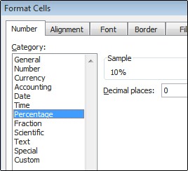
In the Format Cells dialog box, in the Category list, click Percentage.
In the Decimal places box, enter the number of decimal places that you want to display. For example, if you want to see 10% instead of 10.00%, enter 0 in the Decimal places box.

Top of Page

Tips for displaying percentages

To reset the number format of selected cells, click General in the Category list. Cells that are formatted with the General format have no specific number format.
If you want negative percentages to stand out—for example, you want them to appear in red—you can create a custom number format (Format Cells dialog box, Number tab, Custom category). The format should resemble the following: 0.00%;[Red]-0.00%. When applied to cells, this format displays positive percentages in the default text color and negative percentages in red. The portion that follows the semicolon represents the format that is applied to a negative value.

Similarly, you can display negative percentages in parentheses by creating a custom format that looks something like this: 0.00%_);(0.00%). For more information on creating custom formats, see Create or delete a custom number format.
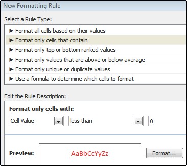
You can also use conditional formatting (Home tab, Styles group, Conditional Formatting) to customize the way negative percentages appear in your workbook. The conditonal formatting rule you create should be similar to the one shown in the following example. This particular rule instructs Excel to apply a format (red text) to a cell if the cell value is less than zero. For more information about conditional formatting, see Add, change, or clear conditional formats.