Format an Excel table

Excel provides numerous predefined table styles that you can use to quickly format a table. If the predefined table styles don't meet your needs, you can create and apply a custom table style. Although you can delete only custom table styles, you can remove any predefined table style so that it is no longer applied to a table.

Example of data formatted as an Excel table

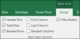
You can further adjust the table formatting by choosing Quick Styles options for table elements, such as Header and Total Rows, First and Last Columns, Banded Rows and Columns, as well as Auto Filtering.

Note: The screen shots in this article were taken in Excel 2016. If you have a different version your view might be slightly different, but unless otherwise noted, the functionality is the same.

Choose a table style

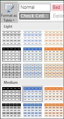
When you have a data range that is not formatted as a table, Excel will automatically convert it to a table when you select a table style. You can also change the format for an existing table by selecting a different format.

Select any cell within the table, or range of cells you want to format as a table.
On the Home tab, click Format as Table.
Click the table style that you want to use.

Notes:

Auto Preview - Excel will automatically format your data range or table with a preview of any style you select, but will only apply that style if you press Enter or click with the mouse to confirm it. You can scroll through the table formats with the mouse or your keyboard's arrow keys.
When you use Format as Table, Excel automatically converts your data range to a table. If you don't want to work with your data in a table, you can convert the table back to a regular range while keeping the table style formatting that you applied. For more information, see Convert an Excel table to a range of data.

Create or delete a custom table style

Important:

Once created, custom table styles are available from the Table Styles gallery under the Custom section.
Custom table styles are only stored in the current workbook, and are not available in other workbooks.

Create a custom table style

Select any cell in the table you want to use to create a custom style.
On the Home tab, click Format as Table, or expand the Table Styles gallery from the Table Tools > Design tab (the Table tab on a Mac).
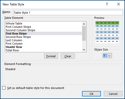
Click New Table Style, which will launch the New Table Style dialog.
In the Name box, type a name for the new table style.
In the Table Element box, do one of the following:
- To format an element, click the element, then click Format, and then select the formatting options you want from the Font, Border or Fill tabs.
- To remove existing formatting from an element, click the element, and then click Clear.
Under Preview, you can see how the formatting changes that you made affect the table.
To use the new table style as the default table style in the current workbook, select the Set as default table style for this document check box.

Delete a custom table style

Select any cell in the table from which you want to delete the custom table style.
On the Home tab, click Format as Table, or expand the Table Styles gallery from the Table Tools > Design tab (the Table tab on a Mac).
Under Custom, right-click the table style that you want to delete, and then click Delete on the shortcut menu.

Note: All tables in the current workbook that are using that table style will be displayed in the default table format.

Remove a table style

Select any cell in the table from which you want to remove the current table style.
On the Home tab, click Format as Table, or expand the Table Styles gallery from the Table Tools > Design tab (the Table tab on a Mac).
Click Clear.

The table will be displayed in the default table format.

Note: Removing a table style does not remove the table. If you don't want to work with your data in a table, you can convert the table to a regular range. For more information, see Convert an Excel table to a range of data.

Choose table style options to format the table elements

There are several table style options that can be toggled on and off. To apply any of these options:

Select any cell in the table.
Go to Table Tools > Design, or the Table tab on a Mac, and in the Table Style Options group, check or uncheck any of the following:
- Header Row - Apply or remove formatting from the first row in the table.
- Total Row - Quickly add SUBTOTAL functions like SUM, AVERAGE, COUNT, MIN/MAX to your table from a drop-down selection. SUBTOTAL functions allow you to include or ignore hidden rows in calculations.
- First Column - Apply or remove formatting from the first column in the table.
- Last Column - Apply or remove formatting from the last column in the table.
- Banded Rows - Display odd and even rows with alternating shading for ease of reading.
- Banded Columns - Display odd and even columns with alternating shading for ease of reading.
- Filter Button - Toggle AutoFilter on and off.

Need more help?

You can always ask an expert in the Excel Tech Community, get support in the Answers community, or suggest a new feature or improvement on Excel User Voice.

Microsoft Office Tutorials

Monday, August 13, 2018