Change the data layout of a Pivottable in Excel 2016 for Windows

After creating a PivotTable and adding the fields to analyze, you can change the layout of the data to make the PivotTable easier to read and scan. Pick a different report layout for instant layout changes.

1. Click anywhere in the PivotTable to show the PivotTable Tools on the ribbon.

   

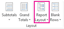
2. Click Design> Report Layout.

   

3. Pick one of the three form options:

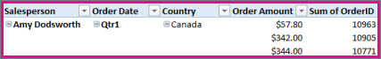
   • Show in Compact Form keeps related data from spreading horizontally off of the screen and minimizes scrolling. This layout is automatically applied when you create a PivotTable.

     

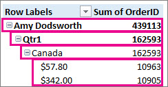
     As shown in the picture above, items from different row area fields are in one column and the items from different fields are indented (like Qtr1 and Canada). Row labels take up less space in compact form, which leaves more room for numeric data. Expand and Collapse buttons are shown so you can display or hide details.

   • Show in Outline Form outlines the data in the PivotTable.

     

     As shown in the picture above, items are outlined in a hierarchy across columns.

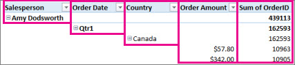
   • Show in Tabular Form shows everything in a table format, which makes it easier to copy cells to another worksheet.

     

     As shown in the picture above, this layout uses one column per field.

4. If you choose outline or tabular form, you can also click Repeat All Item Labels on the Report Layout menu to show item labels for each item.

Tip:  After applying the layout you want, apply a style or banded rows to change the format of the PivotTable using the other options on the Design tab.

Change how subtotals and grand totals are shown

To further refine the layout of the data in your PivotTable, you can change the way subtotals, grand totals, and items are shown.

1. Click anywhere in the PivotTable to show the PivotTable.

2. On the Design tab, do one or more of the following:

   

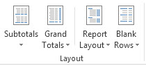
   • Click Subtotals to change how they will be shown for groups of data.

   • Click GrandTotals to change how they will be shown for columns and rows.

   • Click Blank Rows to insert a blank row after each grouping in your PivotTable.

See Also

Create a PivotTable to analyze worksheet data

Sort data in a PivotTable

Filter data in a PivotTable in Excel 2016

Group or ungroup data in a PivotTable report

Search in a PivotTable field list in Excel 2016 for Windows

Turn off time grouping in PivotTables in Excel 2016 for Windows

Use the Field List to arrange fields in a PivotTable in Excel 2016 for Windows

Update (refresh) data in a PivotTable