Use data bars, color scales, and icon sets to highlight data
Important: Some of the content in this topic may not be applicable to some languages.
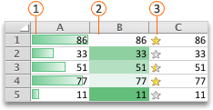
Data bars, color scales, and icon sets are conditional formats that create visual effects in your data. These conditional formats make it easier to compare the values of a range of cells at the same time.

 Data bars
 Color scales
 Icon sets
Format cells by using data bars
Data bars can help you spot larger and smaller numbers, such as top-selling and bottom-selling toys in a holiday sales report. A longer bar represents a larger value, and a shorter bar represents a smaller value.
-
Select the range of cells, the table, or the whole sheet that you want to apply conditional formatting to.
-
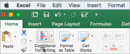
On the Home tab, click Conditional Formatting.

-
Point to Data Bars, and then click a gradient fill or a solid fill.
Tip: When you make a column with data bars wider, the differences between cell values become easier to see.
Format cells by using color scales
Color scales can help you understand data distribution and variation, such as investment returns over time. Cells are shaded with gradations of two or three colors that correspond to minimum, midpoint, and maximum thresholds.
-
Select the range of cells, the table, or the whole sheet that you want to apply conditional formatting to.
-
On the Home tab, click Conditional Formatting.

-
Point to Color Scales, and then click the color scale format that you want.
The top color represents larger values, the center color, if any, represents middle values, and the bottom color represents smaller values.
Format cells by using icon sets
Use an icon set to present data in three to five categories that are distinguished by a threshold value. Each icon represents a range of values and each cell is annotated with the icon that represents that range. For example, a three-icon set uses one icon to highlight all values that are greater than or equal to 67 percent, another icon for values that are less than 67 percent and greater than or equal to 33 percent, and another icon for values that are less than 33 percent.
-
Select the range of cells, the table, or the whole sheet that you want to apply conditional formatting to.
-
On the Home tab, click Conditional Formatting.

-
Point to Icon Sets, and then click the icon set that you want.
Tip: Icon sets can be combined with other conditional formats.
Format cells by using data bars
Data bars can help you spot larger and smaller numbers, such as top-selling and bottom-selling toys in a holiday sales report. A longer bar represents a larger value, and a shorter bar represents a smaller value.
-
Select the range of cells, the table, or the whole sheet that you want to apply conditional formatting to.
-
On the Home tab, under Format, click Conditional Formatting.

-
Point to Data Bars, and then click a gradient fill or a solid fill.
Tip: When you make a column with data bars wider, the differences between cell values become easier to see.
Format cells by using color scales
Color scales can help you understand data distribution and variation, such as investment returns over time. Cells are shaded with gradations of two or three colors that correspond to minimum, midpoint, and maximum thresholds.
-
Select the range of cells, the table, or the whole sheet that you want to apply conditional formatting to.
-
On the Home tab, under Format, click Conditional Formatting.

-
Point to Color Scales, and then click the color scale format that you want.
The top color represents larger values, the center color, if any, represents middle values, and the bottom color represents smaller values.
Format cells by using icon sets
Use an icon set to present data in three to five categories that are distinguished by a threshold value. Each icon represents a range of values and each cell is annotated with the icon that represents that range. For example, a three-icon set uses one icon to highlight all values that are greater than or equal to 67 percent, another icon for values that are less than 67 percent and greater than or equal to 33 percent, and another icon for values that are less than 33 percent.
-
Select the range of cells, the table, or the whole sheet that you want to apply conditional formatting to.
-
On the Home tab, under Format, click Conditional Formatting.

-
Point to Icon Sets, and then click the icon set that you want.
Tip: Icon sets can be combined with other conditional formats.
No comments:
Post a Comment