Split panes to lock rows or columns in separate worksheet areas

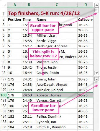
Your friend Tomas finished a 5-K run last weekend, and you want to see the times of the top 10 finishers to compare his time with theirs. You found his name down in row 180 of your spreadsheet. Would you like to know how to see his result together with the top 10 finishers at the top of the worksheet?

By splitting the worksheet, you can scroll down in the lower pane and still see the top rows in the upper pane.

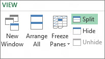
To split this worksheet as shown above, you select below the row where you want the split – selecting row 13 splits the worksheet below row 12. Then, click View > Window > Split. You can remove the split simply by clicking the Split button again.

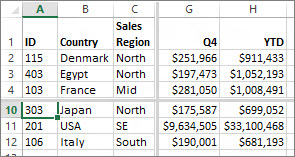
You can also split a worksheet on the columns. Select the column to the right of the column where you want to place the split, and use the Split command. You can also split on both a row and a column. by selecting the cell below and to the right of where you want the split—then click Split. In the figure below—because D5 was chosen—columns to its left (A-C) and rows above it (1-4) are frozen by the split. Then, by selecting a row below row 4 and scrolling up, you no longer see rows 5 through 9. Also, you don't see columns D through F. This brings a tight focus onto Q4 and the YTD totals in columns G and H.

To undo a split, simply click View > Window > Split again.