Sum values based on multiple conditions

If you want to sum values with more than one condition, like the sum of sales of a certain product in a certain region, you'd use the SUMIFS function in a formula.

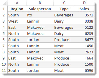
Here's an example where we have two conditions: we want the sum of Meat sales (from column C) in the South region (from column A).

Here's the formula you'd use:

=SUMIFS(D2:D11,A2:A11,"South",C2:C11,"Meat")The result is 14719, and here's how the formula works.

=SUMIFS is an arithmetic formula. It calculates numbers, which in this case are in column D. So start by telling the formula where the numbers are:

• =SUMIFS(D2:D11,

In other words, you want the formula to sum numbers in that column if they meet the conditions. That cell range is your first argument, or piece of data the function needs to run.

Next, you want to find data that meets two conditions, so you enter your first condition by telling the function where the data resides (A2:A11) and what the condition is, which is "South". Notice the commas between the separate arguments.

• =SUMIFS(D2:D11,A2:A11,"South",

Quotation marks around "South" tell Excel it's using text data.

Finally, you enter the arguments for your second condition—the range of cells (C2:C11) that contains the word "meat," plus the word itself (surrounded by quotes) so Excel can match it. End the formula with a closing parenthesis ) and then press Enter to get the result of 14719.

• =SUMIFS(D2:D11,A2:A11,"South",C2:C11,"Meat")

As you type the SUMIFS function, if you don't remember the arguments, help is nearby. After you type =SUMIFS( Formula AutoComplete appears beneath the formula, with the list of arguments in their proper order.

Looking at the image of Formula AutoComplete and the list of arguments, in our example sum_rangeis D2:D11, the column of numbers you want to sum; criteria_range1is A2:A11, the column of data where criteria1 "South" resides.

As you type, the rest of the arguments will appear in Formula AutoComplete; criteria_range2 is C2:C11, the column of data where criteria2 "Meat" resides.

Give it a try

Copy all the data in the table below, and paste into cell A1 in a new worksheet. You may want to adjust column widths to see the formulas better.

Region	Salesperson	Type	Sales
South	Ito	Beverages	3571
West	Lannin	Dairy	3338
East	Makovec	Beverages	5122
North	Makovec	Dairy	6239
South	Jordan	Produce	8677
South	Lannin	Meat	450
South	Lannin	Meat	7673
East	Makovec	Produce	664
North	Lannin	Produce	1500
South	Jordan	Meat	6596
Formula		Description	Result
'=SUMIFS(D2:D11,A2:A11, "South", C2:C11,"Meat")		Sums the Meat Sales in Column C in the South region in Column A (result is 14719).	=SUMIFS(D2:D11,A2:A11, "South", C2:C11,"Meat")