Format negative percentages to make them easy to find

Negative percentages can be difficult to spot when you're scanning a worksheet. You can make them easy to find by applying special formatting to negative percentages—or by creating a conditional formatting rule.

Create a custom format

Follow these steps:

1. Select the cell or cells that contain negative percentages. To select multiple cells, hold down the Ctrl key as you select each cell.

2. On the Home tab, click Format > Format Cells.

   

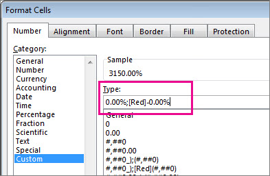
3. In the Format Cells box, in the Category list, click Custom.

4. In the Type box, enter the following format: 0.00%;[Red]-0.00%.

   

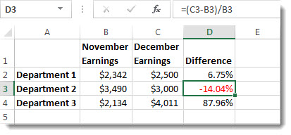
   Now, the negative percentage will appear in red highlighting.

   

   Tip: Custom formats are saved with the workbook. The next time you need to apply it, follow steps 2 and 3 above, and you'll find the custom format in the Type list. To use a custom format in other workbooks, save the workbook as a template, and then base future workbooks on that template.

Create a custom formatting rule

Follow these steps to create a custom formatting rule—which will only be available in the worksheet in which you create it.

1. In a worksheet, select the range of cells in which you'll be entering negative percentages.

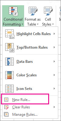
2. On the Home tab, click Conditional Formatting > New Rule. 

   

3. In the New Formatting Rule box, select Format only cells that contain.

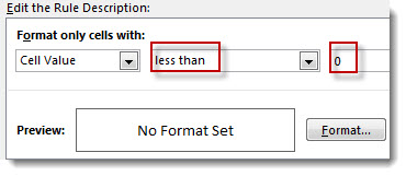
4. In the Edit the Rule Description popup, in Format only cells with, select less than.

   

5. In the field, type the number 0.

6. Click Format.

7. In the Format Cells box, select a font or cell color, and then click OK twice.

When you type a negative percentage within the selected range, it will automatically be formatted in red.

Need more help?

You can always ask an expert in the Excel Tech Community, get support in the Answers community, or suggest a new feature or improvement on Excel User Voice.