Expand, collapse, or show details in a PivotTable or PivotChart
In a PivotTable or PivotChart, you can expand or collapse to any level of data detail, and even for all levels of detail in one operation. You can also expand or collapse to a level of detail beyond the next level. For example, starting at a country/region level, you can expand to a city level which expands both the state/province and city level. This can be a time-saving operation when you work with many levels of detail. In addition, you can expand or collapse all members for each field in an Online Analytical Processing (OLAP) data source.
You can also see the details that are used to aggregate the value in a value field.
Expand or collapse to different levels of detail
In a PivotTable or PivotChart, you can expand or collapse to any level of data detail, and even for all levels of detail in one operation. You can also expand or collapse to a level of detail beyond the next level. For example, starting at a country/region level, you can expand to a city level which expands both the state/province and city level. This can be a time-saving operation when you work with many levels of detail. In addition, you can expand or collapse all members for each field in an OLAP data source.
Expand or collapse levels in a PivotTable
In a PivotTable, do one of the following:
-
Click the expand or collapse button next to the item that you want to expand or collapse.
Note: If you don't see the expand or collapse buttons, see the Show or hide the expand and collapse buttons in a PivotTable section in this topic.
-
Double-click the item that you want to expand or collapse.
-
Right-click (Ctrl+Click on a Mac) the item, click Expand/Collapse, and then do one of the following:
-
To see the details for the current item, click Expand.
-
To hide the details for the current item, click Collapse.
-
To hide the details for all items in a field, click Collapse Entire Field.
-
To see the details for all items in a field, click Expand Entire Field.
-
To see a level of detail beyond the next level, click Expand To "<Field name>".
-
To hide to a level of detail beyond the next level, click Collapse To "<Field name>".
-
Expand or collapse levels in a PivotChart
In a PivotChart, right-click (Ctrl+Click on a Mac) the category label for which you want to show or hide level details, click Expand/Collapse, and then do one of the following:
-
To see the details for the current item, click Expand.
-
To hide the details for the current item, click Collapse.
-
To hide the details for all items in a field, click Collapse Entire Field.
-
To see the details for all items in a field, click Expand Entire Field.
-
To see a level of detail beyond the next level, click Expand To "<Field name>".
-
To hide to a level of detail beyond the next level, click Collapse To "<Field name>".
Show or hide the expand and collapse buttons in a PivotTable
The expand and collapse buttons are displayed by default, but you may have hidden them (for example, when you don't want them to appear in a printed report). To use these buttons to expand or collapse levels of detail in the report, you must make sure that they are displayed.
-
In Excel 2016 and Excel 2013: On the Analyze tab, in the Show group, click +/- Buttons to show or hide the expand and collapse buttons.
-
In Excel 2010: On the Options tab, in the Show group, click +/- Buttons to show or hide the expand and collapse buttons.
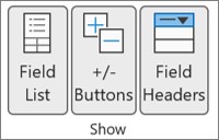
-
In Excel 2007: On the Options tab, in the Show/Hide group, click +/- Buttons to show or hide the expand and collapse buttons.
Note: Expand and collapse buttons are available only for fields that have detail data.
Show or hide details for a value field in a PivotTable
By default, the option to display details for a value field in a PivotTable is turned on. To protect others from seeing this data, you can turn it off.
Show value field details
-
In a PivotTable, do one of the following:
-
Right-click (Ctrl+Click on a Mac) a field in the values area of the PivotTable, and then click Show Details.
-
Double-click a field in the values area of the PivotTable.
The detail data that the value field is based on, is placed on a new worksheet.
-
Hide value field details
-
Right-click (Ctrl+Click on a Mac) the sheet tab of the worksheet that contains the value field data, and then click Hide or Delete.
Disable or enable the option to show value field details
-
Click anywhere in the PivotTable.
-
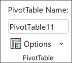
On the Options or Analyze tab (depending on the Excel version you are using) on the ribbon, in the PivotTable group, click Options.
-
In the PivotTable Options dialog box, click the Data tab.
-
Under PivotTable Data, clear or select the Enable show details check box to disable or enable this option.
Note: This setting is not available for an OLAP data source.
Need more help?
You can always ask an expert in the Excel Tech Community, get support in the Answers community, or suggest a new feature or improvement on Excel User Voice.
No comments:
Post a Comment