Create sparklines

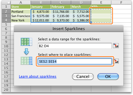
Sparklines are small charts that fit inside individual cells in a sheet. Because of their condensed size, sparklines can reveal patterns in large data sets in a concise and highly visual way. Use sparklines to show trends in a series of values, such as seasonal increases or decreases, economic cycles, or to highlight maximum and minimum values. A sparkline has the greatest effect when it's positioned near the data that it represents. To create sparklines, you must select the data range that you want to analyze, and then select where you want to put the sparklines.

The data range for the sparklines

The location for the sparklines

Column sparklines that display year-to-date sales for Portland, San Francisco, and New York

Newer versions Office for Mac 2011



Create sparklines

1. Select the data range for the sparklines.

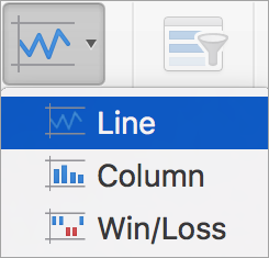
2. On the Insert tab, click Sparklines, and then click the kind of sparkline that you want.

   

   In the Insert Sparklines dialog box, notice that the first box is already filled based on your selection in step 1.

3. On the sheet, select the cell or the range of cells where you want to put the sparklines.

   Important: When you select this area, make sure that you select dimensions that are suitable for the data range. Otherwise, Excel displays errors to indicate that the ranges are not consistent. For example, if the data range has three columns and one row, you should select an adjacent column and the same row.

4. Click OK.

   Tip: When you change the data on the sheet, sparklines update automatically.

Mark data points on sparklines

You can distinguish specific data points, such as high or low values, by using markers.

1. Click a sparkline.

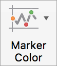
2. On the Sparkline Design tab, in the Show group, select the markers that you want, such as high and low points. You can customize marker colors by clicking the Marker Color button.

   

Change the style of sparklines

1. Click a sparkline.

2. On the Sparkline Design tab, click the style that you want.

   

   To see more styles, point to a style, and then click .

   Tip: To immediately undo a style that you applied, press + Z .

Handle empty or zero value cells

1. Click a sparkline.

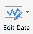
2. On the Sparkline Design tab, click Edit Data, point to Hidden and Empty Cells, and then click the option that you want.

   

Delete sparklines

1. Click the sparkline that you want to delete.

2. On the Sparkline Design tab, click the arrow next to Clear, and then click the option that you want.

   

Create sparklines

1. Select the data range for the sparklines.

2. On the Charts tab, under Insert Sparklines, click the kind of sparkline that you want.

   

   In the Insert Sparklines dialog box, notice that the first box is already filled based on your selection in step 1.

3. On the sheet, select the cell or the range of cells where you want to put the sparklines.

   Important: When you select this area, make sure that you select dimensions that are suitable for the data range. Otherwise, Excel displays errors to indicate that the ranges are not consistent. For example, if the data range has three columns and one row, you should select an adjacent column and the same row.

4. Click OK.

   Tip: When you change the data on the sheet, sparklines update automatically.

Mark data points on sparklines

You can distinguish specific data points, such as high or low values, by using markers.

1. Click a sparkline.

2. On the Sparklines tab, under Markers, select the markers that you want.

Change the style of sparklines

1. Click a sparkline.

2. On the Sparklines tab, under Format, click the style that you want.

   

   To see more styles, point to a style, and then click .

   Tip: To immediately undo a style that you applied, press + Z .

Handle empty or zero value cells

1. Click a sparkline.

2. On the Sparklines tab, under Data, click the arrow next to Edit, point to Hidden and Empty Cells, and then click the option that you want.

   

Delete sparklines

1. Click the sparkline that you want to delete.

2. On the Sparklines tab, under Edit, click the arrow next to Clear, and then click the option that you want.

   

See also

Sparkline axes