Format a date the way you want

When you type something like 2/2 in a cell, Excel knows you're typing a date and formats it based on the date setting in Control Panel. So for example, Excel might format it as 2-Feb. If you change your date setting in Control Panel, the default date format in Excel will change as well. If you don't like the default date format, you can pick a different one in Excel, like February 2, 2012 or 2/2/12. You can also create your own custom format in Excel.

What do you want to do?

Choose from a list of date formats

Create a custom date format

Tips for displaying dates

Choose from a list of date formats

1. Select the cells you want to format.

2. Press CTRL+1.

   On a Mac, press Control+1 or Command+1.

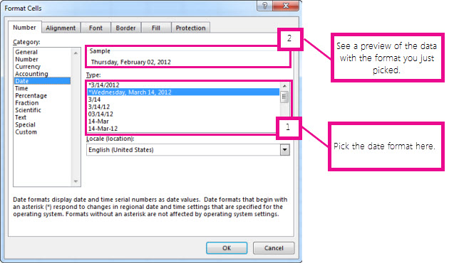
3. In the Format Cells box, click the Number tab.

4. In the Category list, click Date.

1. Under Type, pick a date format. Your format will preview in the Sample box with the first date in your data.

Note:  Date formats that begin with an asterisk (*) will change if you change the regional date and time settings in Control Panel. Formats without an asterisk won't change.

1. If you want to use a date format based on how another language displays dates, pick the language under Locale (location),

   Tip:  Do you have numbers showing up in your cells as #####? This probably means your cell isn't wide enough to show the whole number. Try double-clicking the right border of the column that contains the cells with #####. This will resize the column to fit the number. You can also drag the right border of the column to make it any size you want.

Create a custom date format

If you want to use a format that isn't in the Type box, you can create your own. The easiest way to do this is to start from a format this is close to what you want.

1. Select the cells you want to format.

2. Press CTRL+1.

   On a Mac, press Control+1 or Command+1.

3. In the Format Cells box, click the Number tab.

4. In the Category list, click Date, and then under Type, pick a date format that is close to the format you want.

1. Go back to the Category list, and pick Custom. Under Type, you'll see the format code for the date format you picked in step 4. The built-in date format can't be changed, so don't worry about messing it up. The changes you make will only apply to the custom format you're creating.

2. In the Type box, make the changes you want using code from the table below.

To display	Use this code
Months as 1–12	m
Months as 01–12	mm
Months as Jan–Dec	mmm
Months as January–December	mmmm
Months as the first letter of the month	mmmmm
Days as 1–31	d
Days as 01–31	dd
Days as Sun–Sat	ddd
Days as Sunday–Saturday	dddd
Years as 00–99	yy
Years as 1900–9999	yyyy

If you're modifying a format that includes time values and you use "m" immediately after the "h" or "hh" code or immediately before the "ss" code, Excel displays minutes instead of the month.

Tips for displaying dates

• To quickly use the default date format, click the cell with the date, and then press CTRL+SHIFT+#.

• If a cell displays ##### after you apply date formatting to it, the cell probably isn't wide enough to show the whole number. Try double-clicking the right border of the column that contains the cells with #####. This will resize the column to fit the number. You can also drag the right border of the column to make it any size you want.

• To quickly enter the current date in your worksheet, select any empty cell, press CTRL+; (semicolon), and then press ENTER, if necessary.

• To enter a date that will update to the current date each time you reopen a worksheet or recalculate a formula, type =TODAY() in an empty cell, and then press ENTER.