Summing up ways to add and count Excel data
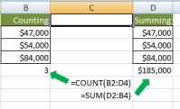
Summing (adding values) is an integral part of data analysis, whether you are subtotaling sales in the Northwest region or doing a running total of weekly receipts. Excel provides multiple techniques that you can use to sum data.
To help you make the best choice, this article provides a comprehensive summary of methods, supporting information to help you quickly decide on which technique to use, and links to in-depth articles.
Summing should not be confused with counting. For more information about counting cells, columns, or rows of data, see Count cells, rows, or columns of data.
In this article
Simple addition and subtraction
You can add and subtract numbers by using a simple formula, clicking a button, or by using a worksheet function.
Add the values in a cell by using a simple formula
If you just need a quick result, you can use Excel as a mini calculator. Do this by using the plus sign (+) arithmetic operator. For example, if you type the formula =5+10 in a cell, Excel displays 15 as the result.
For more information about how to use arithmetic operators in a formula, see the article Use Excel as your calculator.
Subtract the values in a cell by using a simple formula
Do this by using the minus sign (-) arithmetic operator. For example, the formula =12-9 displays a result of 3.
For more information about how to use arithmetic operators in a formula, see the article Use Excel as your calculator.
Add the values in a column or row by using a button
You can use AutoSum to quickly sum a range of numbers in a column or row. Click an empty cell below a column of numbers or to the right of a row of numbers, and then click AutoSum. Excel selects what it determines to be the most likely range of data. Click AutoSum again to accept the range that Excel selects, or select your own range and then click AutoSum.
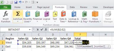
For more information about how to use AutoSum, see the article Use Excel as your calculator.
Add the values in a range by using a function
The SUM function is useful when you want to add or subtract values from different ranges or combine number values with ranges of numbers. Use the SUM function to add all the arguments that you specify within the opening and closing parentheses. Each argument can be a range, a cell reference, or a positive or negative numeric value.
To enter a simple formula, type =SUM in a cell, followed by an opening parenthesis. Next, type one or more numbers, cell references, or cell ranges, separated by commas. Then, type a closing parenthesis and press ENTER to display the result. You can also use your mouse to select cells that contain data that you want to sum.
|
|
For example, using the data in the preceding table, all of the following formulas use the SUM function to return the same value (17158):
-
=SUM(4823,12335)
-
=SUM(A2,A3)
-
=SUM(A2:A3)
-
=SUM(A2,12335)
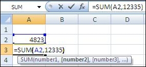
The following figure shows the formula that uses the SUM function to add the value of cell A2 and 12335. Below the formula, a ScreenTip provides guidance for using the SUM function.
Notes:
-
There is no SUBTRACT function in Excel. To subtract values by using a function, use the negative values with the SUM function. For example, the formula =SUM(30,A3,-15,-B6) adds 30 and the value in cell A3, subtracts 15, and also subtracts the value in cell B6.
-
You can include up to 255 numeric values or cell or range references, in any combination, as arguments in the SUM function.
For more information, see the article SUM function.
Subtract the values in a range by using a function
Use the SUM function to subtract numbers by entering the numbers that you want to subtract as negative numbers in the formula.
|
|
For example, using the data in the preceding table, all of the following formulas use the SUM function to return the same value (16737):
-
=SUM(29072,-12335)
-
=SUM(A2,-A3)
-
=SUM(A2,-12335)
-
=SUM(A2,(-1*(A3)))
Summing data by grouping and pivoting
You can use an outline or a PivotTable report to group and summarize your data.
Add the values in a column by using an outline
If your data is in a list and you can logically group it by column values, you can group and summarize data by creating an outline. Creating an outline can summarize data by inserting subtotals and grand totals. Suppose you have the following sales figures, arranged by region and month.
|
|
The following illustration shows an outline with subtotals, grouped by region, and a grand total.
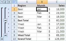
Use the Subtotal command (Data tab, Outline group) to create an outline, subtotals, and a grand total.
The original data included three rows of data for the East region and three rows of data for the West region (rows 2 through 7). Note that the subtotal operation inserted the East Total in row 5 between the last row of East data and the first row of West data.
If you click cell A4 and then click the Subtotal command, Excel creates an outline and inserts rows for East Total, West Total, and Grand Total, and populates the cells in the Sales column with those totals.
For more information, see the following articles:
Outline a list of data in a worksheet
Add the values in a list or Excel table column by using a function
As a more flexible alternative to the Subtotal command, you can use the SUBTOTAL function to calculate subtotals and grand totals on lists or Excel tables that contain hidden rows or columns. In the SUBTOTAL function, you specify an argument that either includes or does not include hidden values.
Note: The SUBTOTAL function can control whether or not hidden rows are included in the results and always ignores rows that have been filtered.
For example, suppose that you want to calculate subtotals and a grand total for data in cells C2 through C7, but you want to ignore the hidden data in row 3 and row 6. The function you use looks like the following:
= SUBTOTAL( 109,C2:C7)
The first argument (109) specifies that you want to add the values in the range and ignore hidden values. To include the hidden values, you instead use 9 as the first argument.
For in-depth information, see the articles SUBTOTAL function and Total the data in an Excel table.
Sum your data and look at it from different perspectives
When a worksheet contains hundreds or even thousands of rows of similar data, it can be difficult to draw meaning from those numbers. You can build a PivotTable report in Excel from that data that shows subtotals, grand totals, and that can summarize data based on categories that you specify.
You can quickly create a PivotTable by selecting a cell in a range of data or Excel table and then, on the Insert tab, in the Tables group, clicking PivotTable.
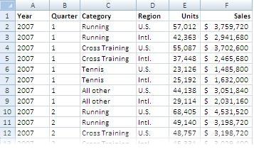
To show the power of a PivotTable, note that in the following example, the sales data contains many rows (there are actually 40 rows of data, but the graphic shows only a portion). In addition, the data isn't summarized, and it has no subtotals or grand total.
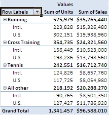
A PivotTable report based on the same data shows subtotals, grand totals, and provides a concise summary at a glance.
Creating and working with PivotTables may require some initial preparation of your data and a familiarity with some concepts.
For detailed information to help you get started, see the following articles:
Calculate values in a PivotTable report
Summing data based on one or more conditions
Using worksheet functions, you can apply conditions (also known as criteria) so that you add only the data that meet conditions that you specify.
Add the values in a range based on a single condition by using a single function or a combination of functions
Use either the SUMIF function or nest the SUM function inside the IF function.
You can add numbers based on a single criterion by using the SUMIF function or by using a combination of the SUM and the IF functions.
For example, the formula =SUMIF(A2:A6,">20") adds only the numbers in the range A2 through A6 that are greater than 20.
Note: The following information is a little bit technical, but definitely worth learning.
If the SUMIF function didn't exist, you could still produce the same answer by combining the IF and the SUM functions. Combining functions in this manner is also known as "nesting," because one function is used in another function.
To create a formula that mimics the SUMIF function, you enter a formula that treats the range A2 through A6 as an array, which means that the range is considered as a single entity containing five cells.
Your formula looks like this: {=SUM(IF(A2:A6>20,A2:A6))}. The "curly" braces that surround the formula indicate that this is an array formula. An array formula requires some special treatment: Instead of typing the braces yourself, you must instead press CTRL+SHIFT+ENTER — Excel then surrounds the formula =SUM(IF(A2:A6>20,A2:A6)) with the braces. If you type the braces yourself, you won't create an array formula.
Try this!
Copy the data from the following table into a worksheet at cell A1. After you paste the data, you'll notice that cell A10 contains a #VALUE! error. This means that you need to convert cell A10 to an array formula. Do this by pressing F2 and then pressing CTRL+SHIFT+ENTER. Excel displays the result (65) in cells A8 and A10.
How to copy the example worksheet data
-
Create a blank workbook or worksheet.
-
Select the example in the Help topic.
Note: Do not select the row or column headers.
 Selecting an example from Help
 -
Press CTRL+C.
-
In the worksheet, select cell A1, and press CTRL+V.
-
To switch between viewing the results and viewing the formulas that return the results, press CTRL+` (grave accent).
|
|
Also, the Knowledge Base article XL: When to Use SUM(IF()) instead of CountBlank() provides additional guidance on when to use the SUMIF function.
Add the values in a column based on single or multiple conditions by using a function
Use the DSUM function to add the numbers in a field (column) of records in a list or database that match conditions (also known as criteria) that you specify.
You can also use the DSUM function when you have a column list and you find it easier to define your conditions in a separate range of cells instead of using a nested function.
For more information, see the article DSUM function.
Add the values in a range based on multiple conditions by using a wizard (for Excel 2007 only)
You can use the Conditional Sum Wizard (Formulas > Solutions >Conditional Sum ) to add values that are based on multiple conditions.
Important: The Conditional Sum Wizard is available only in Excel 2007 and previous versions. For more information, see What happened to the Conditional Sum Wizard add-in?.
If this command is not available (the Solutions group may also not be visible), install and load the Analysis ToolPak add-in.
How to load the Analysis ToolPak
Click the Microsoft Office Button  , click Excel Options, and then click the Add-ins category.
-
In the Manage list, select Excel Add-ins, and then click Go.
-
In the Add-ins available list, select the Analysis ToolPak box, and then click OK.
-
If the wizard appears in the Inactive Application Add-ins list, select the wizard and then click Go to make it active.
-
If necessary, follow the instructions in the Setup program.
To use the Conditional Sum Wizard, select your range of data and click the Conditional Sum command (Solutions group on the Formulas tab). Follow steps 1 through 4 to complete the wizard. The following illustration shows step 2 of the wizard, in which there is one condition: The values to be summed must be greater than 100.

Add the values in a range based on multiple conditions by using a single function or a combination of functions
Use the SUMIFS function. Provide the range that you want to sum, a range that contains conditions, and the conditions that are applied to the conditions range. As an alternative, you can nest the SUM and IF functions.
For more information, see the article SUMIFS function.
Also, see the following Knowledge Base articles for additional information:
Summing squared and array values
You can use worksheet functions to add values in two or more columns that correspond to each other. This type of operation can be as simple as determining a weighted average (see the following example that computes a grade point average), or it can be a complex statistical or engineering calculation.
Sum the product of corresponding values in one or more arrays
Use the SUMPRODUCT function. For example, you can calculate a student's grade point average by using the SUMPRODUCT function and dividing that result by the number of credits, as shown in the following figure.
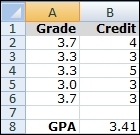
The formula =SUMPRODUCT(A2:A6,B2:B6)/SUM(B2:B6) multiplies the grade achieved for each class by its number of credits, sums those products (61.3), divides that sum by the total credits (18), and determines the grade point average (3.41). This type of calculation is also known as a weighted average.
You can also use the SUMPRODUCT function in more advanced mathematical operations by multiplying several arrays.
The SUMPRODUCT function is easy to use with arrays that have the same dimensions, but you can also use the SUM function in an array formula if you need more flexibility.
For more detailed information, see the article SUMPRODUCT function.
The following four functions are typically used only in advanced statistical or complex mathematical applications, so only a brief description is provided. For more information, click the function name to go directly to its reference topic.
-
SUMSQ function Returns the sum of the squares of a list of numbers or values in a range. For example, SUMSQ(2,3) returns 13.
-
SUMX2PY2 function Adds the sum of the squares of corresponding values in two arrays.
-
SUMX2MY2 function Returns the sum of the difference of squares of corresponding values in two arrays.
-
SUMXMY2 function Returns the sum of squares of differences of corresponding values in two arrays.
Special cases (running total, unique values)
You can use worksheet functions to create totals that are automatically updated as you add more data to a range or table, or to add only the unique values that are found in a range or table.
Create a running total by using a function
Use the SUM function. For example, create column headings in a worksheet named Deposits, Withdrawals, and Balance.
-
In the first cell under the Balance column, enter your beginning balance.
-
In the cell directly below your balance (in this case, C3), enter a formula that adds the value from the Deposits column in the same row and subtracts the value from the Withdrawals column (=SUM(C2,A3,-B3).
-
Drag this formula down to any new rows that you add. In the following example, it is dragged to row 4.
The example may be easier to understand if you copy it to a blank worksheet.
How to copy an example
-
Create a blank workbook or worksheet.
-
Select the example in the Help topic.
Note: Do not select the row or column headers.

Selecting an example from Help
-
Press CTRL+C.
-
In the worksheet, select cell A1, and press CTRL+V.
-
To switch between viewing the results and viewing the formulas that return the results, press CTRL+` (grave accent), or on the Formulas tab, in the Formula Auditing group, click the Show Formulas button.
-
|
|
You can use a running balance as you would use a check register to watch values of items in cells increase or decrease as you enter new items and values over time.
For more information, see the article Calculate a running balance.
Add the unique values in a range by using a compound formula
In a column, enter a list of values that contains duplicates, and then use a combination of the SUM, IF, and FREQUENCY functions to add only the unique values that are found in that range.
Including values from other worksheets or workbooks in a formula
You can add or subtract cells or ranges of data from other worksheets or workbooks in a formula by including a reference to them. To refer to a cell or range in another worksheet or workbook, use instructions in the following table.
| To refer to: | Enter this | Examples |
| A cell or range in another worksheet in the same workbook | The name of the worksheet followed by an exclamation point, followed by the cell reference or range name. | Sheet2!B2:B4 |
| A cell or range in another workbook that is currently open | The file name of the workbook in brackets ([]) and the name of the worksheet followed by an exclamation point, followed by the cell reference or range name. | [MyWorkbook.xlsx]Sheet1!A7 |
| A cell or range in another workbook that is not open | The full path and file name of the workbook in brackets ([]) and the name of the worksheet followed by an exclamation point, followed by the cell reference or range name. If the full path contains any space characters, surround the start of the path and the end of the worksheet name with single quotation marks (see the example). | ['C:\My Documents\[MyWorkbook.xlsx]Sheet1'!A2:A5 |
Summing and subtracting date and time values
You can use date and time functions and even simple addition or subtraction to calculate elapsed time, estimate completion dates for projects, and more. The following table shows some formulas that calculate elapsed times and days. Note that if you subtract a date or time that results in a negative value, Excel displays ### characters in the cell that contains the formula.
The example may be easier to understand if you copy it to a blank worksheet.
How to copy an example
-
Create a blank workbook or worksheet.
-
Select the example in the Help topic.
Note: Do not select the row or column headers.

Selecting an example from Help
-
Press CTRL+C.
-
In the worksheet, select cell A1, and press CTRL+V.
-
To switch between viewing the results and viewing the formulas that return the results, press CTRL+` (grave accent), or on the Formulas tab, in the Formula Auditing group, click the Show Formulas button.
|
|
Working with date and time values can produce unexpected results, so proceed carefully.
Displaying calculations on the Excel status bar
For a quick look at totals of cells that are selected in your worksheet, take a look at the Excel status bar (the status bar is at the bottom of the document window).
When one or more cells are selected, information about the data in those cells is displayed on the Excel status bar. For example, if four cells on your worksheet are selected, and they contain the values 2, 3, a text string (such as "cloud"), and 4, all of the following values can be displayed on the status bar at the same time: Average, Count, Numerical Count, Min, Max, and Sum. Right-click the status bar to show or hide any or all of these values. These values are shown in the illustration that follows.

No comments:
Post a Comment