Apply color to alternate rows or columns

Adding a color to alternate rows or columns (often called color banding) can make the data in your worksheet easier to scan. To format alternate rows or columns, you can quickly apply a preset table format. By using this method, alternate row or column shading is automatically applied when you add rows and columns.

Here's how:

1. Select the range of cells that you want to format.

2. Click Home > Format as Table.

3. Pick a table style that has alternate row shading.

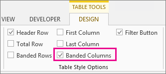
4. To change the shading from rows to columns, select the table, click Design, and then uncheck the Banded Rows box and check the Banded Columns box.

   

Tip: If you want to keep a banded table style without the table functionality, you can convert the table to a data range. Color banding won't automatically continue as you add more rows or columns but you can copy alternate color formats to new rows by using Format Painter.

Use conditional formatting to apply banded rows or columns

You can also use a conditional formatting rule to apply different formatting to specific rows or columns.

Here's how:

1. On the worksheet, do one of the following:

   • To apply the shading to a specific range of cells, select the cells you want to format.

   • To apply the shading to the whole worksheet, click the Select All button.

     

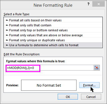
2. Click Home > Conditional Formatting > New Rule.

   

3. In the Select a Rule Type box, click Use a formula to determine which cells to format.

4. To apply color to alternate rows, in the Format values where this formula is true box, type the formula =MOD(ROW(),2)=0.

   To apply color to alternate columns, type this formula: =MOD(COLUMN(),2)=0.

   These formulas determine whether a row or column is even or odd numbered, and then applies the color accordingly.

5. Click Format.

6. In the Format Cells box, click Fill.

7. Pick a color and click OK.

8. You can preview your choice under Sample and click OK or pick another color.

   Tips: 

   • To edit the conditional formatting rule, click one of the cells that has the rule applied, click Home > Conditional Formatting > Manage Rules > Edit Rule, and then make your changes.

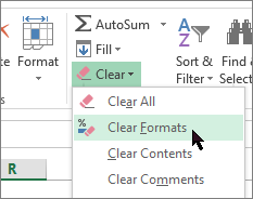
   • To clear conditional formatting from cells, select them, click Home > Clear, and pick Clear Formats.

     

   • To copy conditional formatting to other cells, click one of the cells that has the rule applied, click Home > Format Painter , and then click the cells you want to format.