You can use a PivotTable to summarize, analyze, explore, and present summary data. PivotCharts complement PivotTables by adding visualizations to the summary data in a PivotTable, and allow you to easily see comparisons, patterns, and trends. Both PivotTables and PivotCharts enable you to make informed decisions about critical data in your enterprise. You can also connect to external data sources such as SQL Server tables, SQL Server Analysis Services cubes, Azure Marketplace, Office Data Connection (.odc) files, XML files, Access databases, and text files to create PivotTables, or use existing PivotTables to create new tables.
Note: The screen shots in this article were taken in Excel 2016. If you have a different version your view might be slightly different, but unless otherwise noted, the functionality is the same.
About PivotTables
A PivotTable is an interactive way to quickly summarize large amounts of data. You can use a PivotTable to analyze numerical data in detail, and answer unanticipated questions about your data. A PivotTable is especially designed for:
-
Querying large amounts of data in many user-friendly ways.
-
Subtotaling and aggregating numeric data, summarizing data by categories and subcategories, and creating custom calculations and formulas.
-
Expanding and collapsing levels of data to focus your results, and drilling down to details from the summary data for areas of interest to you.
-
Moving rows to columns or columns to rows (or "pivoting") to see different summaries of the source data.
-
Filtering, sorting, grouping, and conditionally formatting the most useful and interesting subset of data enabling you to focus on just the information you want.
-
Presenting concise, attractive, and annotated online or printed reports.
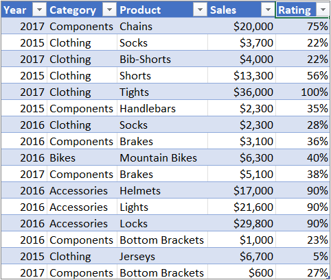
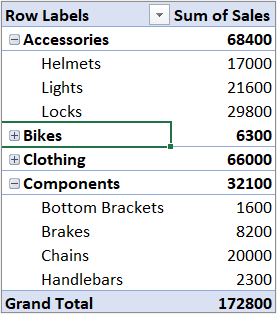
For example, here's a simple list of household expenses on the left, and a PivotTable based on the list to the right:
| Household expense data | Corresponding PivotTable |
| | |
For more information, see Create a PivotTable to analyze worksheet data.
Ways to work with a PivotTable
After you create a PivotTable by selecting its data source, arranging fields in the PivotTable Field List, and choosing an initial layout, you can perform the following tasks as you work with a PivotTable:
Explore the data by doing the following:
-
Expand and collapse data, and show the underlying details that pertain to the values.
-
Sort, filter, and group fields and items.
-
Change summary functions, and add custom calculations and formulas.
Change the form layout and field arrangement by doing the following:
-
Change the PivotTable form: Compact, Outline, or Tabular.
-
Add, rearrange, and remove fields.
-
Change the order of fields or items.
Change the layout of columns, rows, and subtotals by doing the following:
-
Turn column and row field headers on or off, or display or hide blank lines.
-
Display subtotals above or below their rows.
-
Adjust column widths on refresh.
-
Move a column field to the row area or a row field to the column area.
-
Merge or unmerge cells for outer row and column items.
Change the display of blanks and errors by doing the following:
-
Change how errors and empty cells are displayed.
-
Change how items and labels without data are shown.
-
Display or hide blank rows
Change the format by doing the following:
-
Manually and conditionally format cells and ranges.
-
Change the overall PivotTable format style.
-
Change the number format for fields.
-
Include OLAP Server formatting.
For more information, see Design the layout and format of a PivotTable.
About PivotCharts
PivotCharts provide graphical representations of the data in their associated PivotTables. PivotCharts are also interactive. When you create a PivotChart, the PivotChart Filter Pane appears. You can use this filter pane to sort and filter the PivotChart's underlying data. Changes that you make to the layout and data in an associated PivotTable are immediately reflected in the layout and data in the PivotChart and vice versa.
PivotCharts display data series, categories, data markers, and axes just as standard charts do. You can also change the chart type and other options such as the titles, the legend placement, the data labels, the chart location, and so on.
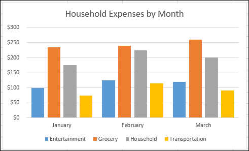
Here's a PivotChart based on the PivotTable example above.

For more information, see Create a PivotChart.
Differences between PivotCharts and standard charts
If you are familiar with standard charts, you will find that most operations are the same in PivotCharts. However, there are some differences:
Row/Column orientation Unlike a standard chart, you cannot switch the row/column orientation of a PivotChart by using the Select Data Source dialog box. Instead, you can pivot the Row and Column labels of the associated PivotTable to achieve the same effect.
Chart types You can change a PivotChart to any chart type except an xy (scatter), stock, or bubble chart.
Source data Standard charts are linked directly to worksheet cells, while PivotCharts are based on their associated PivotTable's data source. Unlike a standard chart, you cannot change the chart data range in a PivotChart's Select Data Source dialog box.
Formatting Most formatting—including chart elements that you add, layout, and style—is preserved when you refresh a PivotChart. However, trendlines, data labels, error bars, and other changes to data sets are not preserved. Standard charts do not lose this formatting once it is applied.
Although you cannot directly resize the data labels in a PivotChart, you can increase the text font size to effectively resize the labels.
Creating a PivotTable or PivotChart from worksheet data
You can use data from a Excel worksheet as the basis for a PivotTable or PivotChart. The data should be in list format, with column labels in the first row, which Excel will use for Field Names. Each cell in subsequent rows should contain data appropriate to its column heading, and you shouldn't mix data types in the same column. For instance, you shouldn't mix currency values and dates in the same column. Additionally, there shouldn't be any blank rows or columns within the data range.
Excel tables Excel tables are already in list format and are good candidates for PivotTable source data. When you refresh the PivotTable, new and updated data from the Excel table is automatically included in the refresh operation.
Using a dynamic named range To make a PivotTable easier to update, you can create a dynamic named range, and use that name as the PivotTable's data source. If the named range expands to include more data, refreshing the PivotTable will include the new data.
Including totals Excel automatically creates subtotals and grand totals in a PivotTable. If the source data contains automatic subtotals and grand totals that you created by using the Subtotals command in the Outline group on the Data tab, use that same command to remove the subtotals and grand totals before you create the PivotTable.
Using an external data source to create a PivotTable or PivotChart
You can retrieve data from an external data source such as a database, an Online Analytical Processing (OLAP) cube, or a text file. For example, you might maintain a database of sales records you want to summarize and analyze.
Office Data Connection files If you use an Office Data Connection (ODC) file (.odc) to retrieve external data for a PivotTable, you can input the data directly into a PivotTable. We recommend that you retrieve external data for your reports by using ODC files.
OLAP source data When you retrieve source data from an OLAP database or a cube file, the data is returned to Excel only as a PivotTable or a PivotTable that has been converted to worksheet functions. For more information, see Convert PivotTable cells to worksheet formulas.
Non-OLAP source data This is the underlying data for a PivotTable or a PivotChart that comes from a source other than an OLAP database. For example, data from relational databases or text files.
For more information, see Create a PivotTable with an external data source.
Using another PivotTable as a data source
The PivotTable cache Each time that you create a new PivotTable or PivotChart, Excel stores a copy of the data for the report in memory, and saves this storage area as part of the workbook file - this is called the PivotTable cache. Each new PivotTable requires additional memory and disk space. However, when you use an existing PivotTable as the source for a new one in the same workbook, both share the same cache. Because you reuse the cache, the workbook size is reduced and less data is kept in memory.
Location requirements To use one PivotTable as the source for another, both must be in the same workbook. If the source PivotTable is in a different workbook, copy the source to the workbook location where you want the new one to appear. PivotTables and PivotCharts in different workbooks are separate, each with its own copy of the data in memory and in the workbooks.
Changes affect both PivotTables When you refresh the data in the new PivotTable, Excel also updates the data in the source PivotTable, and vice versa. When you group or ungroup items, or create calculated fields or calculated items in one, both are affected. If you need to have a PivotTable that's independent of another one, then you can create a new one based on the original data source, instead of copying the original PivotTable. Just be mindful of the potential memory implications of doing this too often.
PivotCharts You can base a new PivotTable or PivotChart on another PivotTable, but you cannot base a new PivotChart directly on another PivotChart. Changes to a PivotChart affect the associated PivotTable, and vice versa.
Changing the source data of an existing PivotTable
Changes in the source data can result in different data being available for analysis. For example, you may want to conveniently switch from a test database to a production database. You can update a PivotTable or a PivotChart with new data that is similar to the original data connection information by redefining the source data. If the data is substantially different with many new or additional fields, it may be easier to create a new PivotTable or PivotChart.
Displaying new data brought in by refresh Refreshing a PivotTable can also change the data that is available for display. For PivotTables based on worksheet data, Excel retrieves new fields within the source range or named range that you specified. For reports based on external data, Excel retrieves new data that meets the criteria for the underlying query or data that becomes available in an OLAP cube. You can view any new fields in the Field List and add the fields to the report.
Changing OLAP cubes that you create Reports based on OLAP data always have access to all of the data in the cube. If you created an offline cube that contains a subset of the data in a server cube, you can use the Offline OLAP command to modify your cube file so that it contains different data from the server.
Need more help?
You can always ask an expert in the Excel Tech Community, get support in the Answers community, or suggest a new feature or improvement on Excel User Voice.


No comments:
Post a Comment