Show or hide subtotals and totals in a PivotTable with Excel 2016 for Mac

When you create a PivotTable that shows value amounts, subtotals and grand totals appear automatically, but you can also show or hide them.

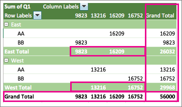
Tip: Row grand totals are only displayed if your data just has one column, because a grand total for a group of columns often doesn't make sense (for example, if one column contains quantities and one column contains prices). If you want to display a grand total of data from several columns, create a calculated column in your source data, and display that column in your PivotTable.

Show or hide subtotals

To show or hide subtotals:

1. Click anywhere in the PivotTable to show the PivotTable Analyze and Design tabs.

   

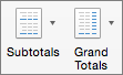
2. Click Design > Subtotals.

   

3. Pick the option you want:

   • Don't Show Subtotals

   • Show All Subtotals at Bottom of Group

   • Show All Subtotals at Top of Group

     Tip:  You can include filtered items in the total amounts by clicking Include Filtered Items in Totals. Click this option again to turn it off.

Show or hide grand totals

1. Click anywhere in the PivotTable to show the PivotTable Analyze and Design tabs.

   

2. Click Design > Grand Totals.

   

3. Pick the option you want:

   • Off for Rows & Columns

   • On for Rows & Columns

   • On for Rows Only

   • On for Columns Only