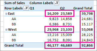
Show or hide subtotals and totals in a PivotTable in Excel 2016 for Windows

When you create a PivotTable that shows value amounts, subtotals and grand totals appear automatically, but you can hide them.

Show or hide subtotals

1. Click anywhere in the PivotTable to show the PivotTable Tools.

   

2. Click Design > Subtotals, and pick the option you want.

   

   Tip:  You can include filtered items in the total amounts by clicking Include Filtered Items in Totals. Click this option again to turn it off. You'll find additional options for totals and filtered items on the Totals & Filters tab in the PivotTable Options box (Analyze > Options).

Show or hide grand totals

1. Click anywhere in the PivotTable to show the PivotTable Tools on the ribbon.

   

2. Click Design > Grand Totals, and pick the option you want.

   

   Tip:  If you don't want to show grand totals for rows or columns, uncheck the Show grand totals for rows or Show grand totals for columns boxes on the Totals & Filters tab in the PivotTable Options box (Analyze > Options).

See Also

Create a PivotTable in Excel 2016 to analyze worksheet data

Filter data in a PivotTable in Excel 2016

Group or ungroup data in a PivotTable report

Turn off time grouping in PivotTables in Excel 2016 for Windows