Freeze panes to lock rows and columns
To keep an area of a worksheet visible while you scroll to another area of the worksheet, go to the View tab, where you can Freeze Panes to lock specific rows and columns in place, or you can Split panes to create separate windows of the same worksheet.
Freezing panes versus splitting panes
When you freeze panes, Microsoft Excel keeps specific rows or columns visible when you scroll in the worksheet. For example, if the first row in your spreadsheet contains headers, you might freeze that row to make sure that the column headers remain visible as you scroll down in your spreadsheet.

A solid line under row 1 indicates that the row is frozen to keep column headers in place when you scroll.
Splitting panes is a variation on freezing panes, in that when you split panes, Excel creates either two or four separate worksheet areas that you can scroll within, while rows or columns in the non-scrolled area remain visible.
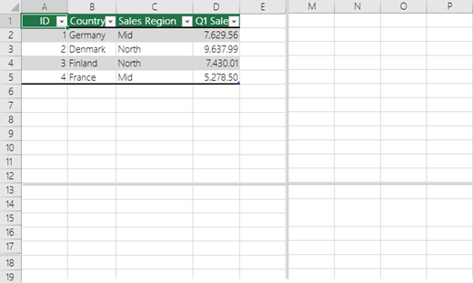
For more information, see Split panes to lock rows or columns in separate worksheet areas.
Note: You cannot freeze panes and split panes at the same time. You can enable only one of the two.
Freeze rows or columns
Before you choose to freeze rows or columns in a worksheet, it's important to consider the following:
-
You can freeze only rows at the top and columns on the left side of the worksheet. You cannot freeze rows and columns in the middle of the worksheet.
-
The Freeze Panes command is not available when you're in cell editing mode (that is, you're entering a formula or data in a cell) or when a worksheet is protected. To cancel cell editing mode, press Enter or Esc.
You can choose to freeze just the top row of your worksheet, just the left column of your worksheet, or multiple rows and columns simultaneously. For example, if you freeze row 1 and then decide to freeze column A, row 1 will no longer be frozen. If you want to freeze both rows and columns, you need to freeze them at the same time.
-
Do one of the following:
-
To lock one row only, choose the View tab, and then click Freeze Top Row.
-
To lock one column only, choose the View tab, and then click Freeze First Column.
-
To lock more than one row or column, or to lock both rows and columns at the same time, choose the View tab, and then click Freeze Panes. You will want your cursor to be below the row(s) you want to freeze and to the right of any column(s) you want to freeze.
-
To lock multiple rows (starting with row 1), select the row below the last row you want frozen, choose the View tab, and then click Freeze Panes.
-
To lock multiple columns, select the column to the right of the last column you want frozen, choose the View tab, and then click Freeze Panes.
-
Note: If you don't see the View tab, it's likely that you are using Excel Starter. To learn more about features that aren't supported in that version, see Excel features that are not fully supported in Excel Starter.
Watch Now

Freeze the top row and the first column at the same time
To freeze the top row and the first column at the same time, click the View tab > Freeze Panes > Freeze Panes.
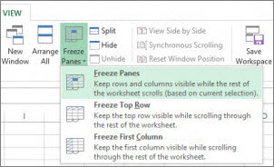
Freeze the top row
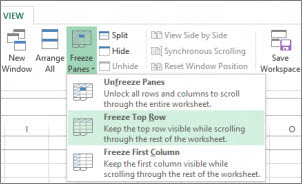
Notice that the border under row 1 is a little darker than other borders, meaning that the row above it is frozen.

Freeze the first column
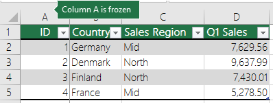
If you'd rather freeze the leftmost column instead, click the View tab > Freeze Panes > Freeze First Column.
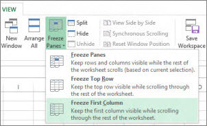
Now, the line to the right of column A is a little darker than the other lines, meaning that the column to its left is frozen.
Unfreeze rows or columns
-
On the View tab > Window > Unfreeze Panes.

Note: If you don't see the View tab, it's likely that you are using Excel Starter. To learn more about features that aren't supported in that version, see Excel features that are not fully supported in Excel Starter.
Do you have a specific question?
Help us improve Excel
Do you have suggestions about how we can improve the next version of Excel? If so, please check out the topics at Excel User Voice.
No comments:
Post a Comment