Apply conditional formatting in Excel

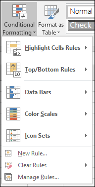
Conditional formatting allows you to apply colors to cells based on certain conditions, like duplicate values, values that meet certain criteria, like greater than 100, or equals "Revenue" with Highlight Cells Rules and Top/Bottom Rules. You can also show how individual cells rank against a range of values with Data Bars, Color Scales and Icon Sets. Conditional formatting is dynamic, so as your values change, the formatting will automatically adjust.

Conditional formatting options	Conditional formatting with Color Scales

Note: Prior to Excel 2007, conditional formatting rules needed to be created with a formula, and only supported three levels. Since Excel 2007, conditional formatting has many pre-defined rules that are easy to apply, and can support up to 64 levels. If you have a formatting situation that can't be created with the pre-defined conditional formats, then you can still use a formula to apply conditional formatting.

In this topic, we'll demonstrate several methods of applying some of these pre-defined conditional formatting rules. Just be aware that there are thousands of different combinations you can create, so you should experiment with them until you find what works best for you. You should also be thoughtful of your audience, as it's not hard to apply so many different conditional formats that you make it difficult for someone to figure out what you're trying to show.

Highlight duplicate values with color

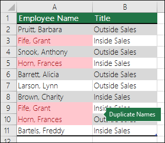
You can highlight duplicate items in a column of data:

1. Pick the range where you want to format duplicate values with a color, like the Employee Name column in this case.

2. On the Home tab, click Conditional Formatting > Highlight Cells Rules > Duplicate Values.

   

3. Select a format from the options drop-down list, then click OK to format the cells.

   

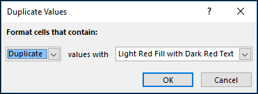
Now the range is formatted with duplicate items highlighted in the color you selected.

Sort by color

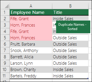
You can take your duplicate search a step farther by sorting your list by color. This can make it easier to apply bulk changes to the duplicates, like deleting them.

1. Click anywhere in your data range, and on the Data tab, click Sort & Filter > Sort.

2. Select Employee Name for the Sort by option, Sort On > Cell Color, then Order > Select the Sort color > On Top, and click OK.

The sorted table will group the duplicates at the top:

Highlight the Top 10 items in a range

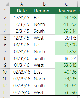
The Top 10 Items option can quickly identify the top performers in a range, like the top 10 customers in a list based on rank. Similarly, you could also choose the Bottom 10 Items, Top/Bottom 10%, or Above/Below Average. You can change the 10 to whatever value you want once you've selected a rule. In the following example, we're highlighting the top 10 revenue performances.

1. Select the range you want to format. In the example above it's the Revenue column.

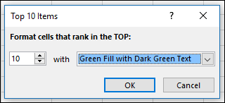
2. On the Home tab, click Conditional Formatting > Top/Bottom Rules > Top 10 Items.

   

3. You can then adjust the number of options you want up or down, and the fill color.

   

Show variances with Data Bars

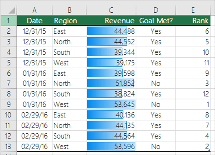
When you use conditional formatting to show Data Bars, Excel draws a bar in each cell whose length corresponds to the value of the cell relative to the other cells in the selected range.

1. Select the range that you want to format. In this case, it's the Revenue column.

2. On the Home tab, click Conditional Formatting > Data Bars > Select the Gradient or Solid Fill style of your choice.

   

3. If you want to sort the list after applying your data bars, just select the column, and on the Data tab, click Sort & Filter, then select either the or option to sort in ascending or descending order.

Highlight positive, neutral and negative values with Icon Sets

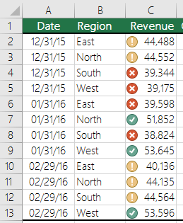
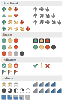
Using a set of icons, you can visually indicate where values fall within certain ranges on a number or percent scale. In the following example, we're showing regional performance to a goal with positive , neutral , and negative icons.

1. Select the range you want to format.

2. On the Home tab, click Conditional Formatting > Icon Sets > select the icon set style of your choice.

   

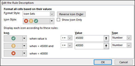
3. Excel will try to interpret your data and format accordingly, but if you want to change it, you can go to the Home tab, click Conditional Formatting > Manage Rules > select the Icon Set Rule > Edit Rule. Then adjust the "Display each icon according to these rules" section. In this case, we're setting the rule so that anything greater than 45,000 is positive, anything between 40,000 and 45,000 is neutral, and anything less than 40,000 is negative.

   

Show variances with Color Scales

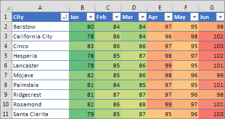
Using Color Scales, you can highlight values to show a range and compare highs and lows, in this case Jan-Jun.

1. Select the range that has the values you want to format.

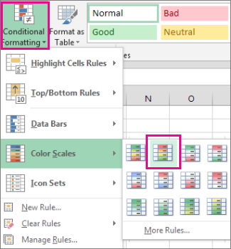
2. On the Home tab, click Conditional Formatting > Color Scales > select the scale of your choice. In this case, we used the Red – Yellow - Green Color Scale .

   

Formatting every other row with a table

If you'd like to apply formatting to every other row in your data, you can do that with a conditional formatting formula, but it's much easier to simply format your data as a table. Select a cell within your data range and go to Home > Styles > Format as Table > select the style of your choice from the Style Gallery, and Excel will instantly transform your data into a table.

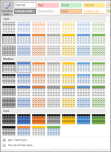
If you only want the table formatting, but not the additional functionality of a table, you can convert the table back to a range. Click anywhere within the table range, then click the Table Tools tab on the Ribbon > Design > Tools > Convert to Range.

You can learn more about Excel Tables here: Create or delete an Excel table in a worksheet.

Looking for something else?

If none of the above options is what you're looking for, you can create your own conditional formatting rule.

1. Pick the cells you want to format.

2. On the Home tab, click Conditional Formatting > New Rule.

   

3. Create your rule and specify its format options, then click OK. You can also see Use a formula to apply conditional formatting for more details.

Need more help?

You can always ask an expert in the Excel Tech Community, get support in the Answers community, or suggest a new feature or improvement on Excel User Voice.

See Also

Quick start: Apply conditional formatting

Use a formula to apply conditional formatting

Using conditional formatting to highlight dates in Excel