Sort data in a pivottable

To help you locate data that you want to analyze in a PivotTable more easily, you can sort text entries (from A to Z or Z to A), numbers (from smallest to largest or largest to smallest), and dates and times (from oldest to newest or newest to oldest).

When you sort data in a PivotTable, be aware of the following:

• Sort orders vary by locale setting. Make sure that you have the correct locale setting in Language and Text in System Preferences on your computer. For information about changing the locale setting, see the Mac Help system.

• Data such as text entries may have leading spaces that affect the sort results. For optimal sort results, you should remove any spaces before you sort the data.

• Unlike sorting data in a range of cells on a worksheet or in an Excel for Mac table, you can't sort case-sensitive text entries.

• You can't sort data by a specific format, such as cell or font color, or by conditional formatting indicators, such as icon sets.

Newer versions Office 2011



Sort row or column label data in a PivotTable

1. In the PivotTable, click any field in the column that contains the items that you want to sort.

2. On the Data tab, click Sort, and then click the sort order that you want. For additional sort options, click Options.

   

   Text entries will be sorted in alphabetical order, numbers will be sorted from smallest to largest (or vice versa), and dates or times will be sorted from oldest to newest (or vice versa).

   Note: You can also quickly sort data in ascending or descending order by clicking A to Z or Z to A. When you do this, text entries are sorted from A to Z or from Z to A, numbers are sorted from smallest to largest or from largest to smallest, and dates or times are sorted from oldest to newest or newest to oldest.

Sort on an individual value

You can sort on individual values or on subtotals by right-clicking a cell, clicking Sort, and choosing a sort method. The sort order is applied to all the cells at the same level in the column that contains the cell.

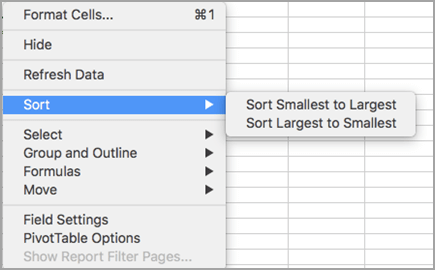
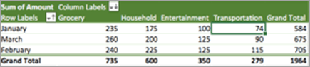
In the example shown below, the data in the Transportation column is sorted smallest to largest.

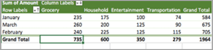
To see the grand totals sorted largest to smallest, choose any number in the Grand Total row or column, and then click Sort > Largest to Smallest.

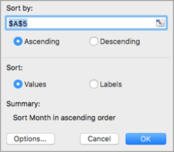
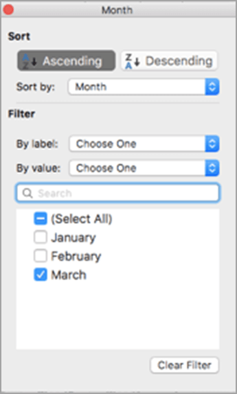
Set custom sort options

To sort specific items manually or change the sort order, you can set your own sort options.

1. Click a field in the row or column you want to sort.

2. Click the arrow next to Row Labels or Column Labels.

   

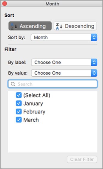
3. Under Sort, choose Ascending or Descending, and select from the options in the Sort by list. (These options will vary based on the your selections in steps 1 and 2.)

4. Under Filter, select any other criteria you might have. For example, if you wanted to see the data for March only, in the By label list, select Equals and then type March in the text box that appears. To include only certain data in your calculations, select or clear the the check boxes in the Filter box. To undo your selection, click Clear Filter.

   <insert sort6 & sort7>

   

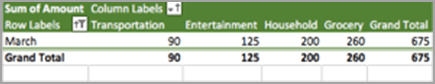
5. Click outside the custom sort dialog box to close it.

Sort row or column label data in a PivotTable

1. In the PivotTable, click any field in the column that contains the items that you want to sort.

2. On the Data tab, under Sort & Filter, click the arrow next to Sort, and then click the sort order that you want.

   Note: You can also quickly sort data in ascending or descending order by clicking A to Z or Z to A. When you do this, text entries are sorted from A to Z or from Z to A, numbers are sorted from smallest to largest or from largest to smallest, and dates or times are sorted from oldest to newest or newest to oldest.

Customize the sort operation

1. Select a cell in the column that you want to sort by.

2. On the Data tab, under Sort & Filter, click the arrow next to Sort, and then click Custom Sort.

3. Configure the type of sort that you want.

Sort by using a custom list

You can sort in a user-defined sort order by using a custom list.

1. Select a cell in the column that you want to sort by.

2. On the Data tab, under Sort & Filter, click the arrow next to Sort, and then click Custom Sort.

3. Click Options.

4. Under First key sort order, select the custom list that you want to sort by.

   Excel provides built-in day-of-the-week and month-of-the year custom lists. You can also create your own custom list. A custom list sort order is not retained when you refresh the PivotTable.

   Note: Custom lists are enabled by default. Disabling custom lists may improve performance when you sort large amounts of data. To disable custom lists, follow these steps:

   1. On the PivotTable tab, click Options, click PivotTable Options, and then click Layout.

   2. In the Sort area, clear the Use custom lists when sorting check box.

Sort data in the values area

1. In a PivotTable, select a value field.

2. On the Data tab, under Sort & Filter, do one or both of the following:

   • To quickly sort in ascending or descending order, click A to Z or Z to A. Numbers are sorted smallest to largest or largest to smallest.

   • To customize the sort operation, click the arrow next to Sort, click Custom Sort, and then configure the type of sort that you want.