Format numbers as currency
If you want to display numbers as monetary values, you must format those numbers as currency. To do this, you apply either the Currency or Accounting number format to the cells that you want to format. The number formatting options are available on the Home tab, in the Number group.

In this article
Format numbers as currency
You can display a number with the default currency symbol by selecting the cell or range of cells, and then clicking Accounting Number Format  in the Number group on the Home tab. (If you want to apply the Currency format instead, select the cells, and press Ctrl+Shift+$.)
If you want more control over either format, or you want to change other aspects of formatting for your selection, you can follow these steps.
Select the cells you want to format
On the Home tab, click the Dialog Box Launcher next to Number.

Tip: You can also press Ctrl+1 to open the Format Cells dialog box.
In the Format Cells dialog box, in the Category list, click Currency or Accounting.

In the Symbol box, click the currency symbol that you want.
Note: If you want to display a monetary value without a currency symbol, you can click None.
In the Decimal places box, enter the number of decimal places that you want for the number. For example, to display $138,691 instead of $138,690.63 in the cell, enter 0 in the Decimal places box.
As you make changes, watch the number in the Sample box. It shows you how changing the decimal places will affect the display of a number.
In the Negative numbers box, select the display style you want to use for negative numbers. If you don't want the existing options for displaying negative numbers, you can create your own number format. For more information about creating custom formats, see Create or delete a custom number format.
Note: The Negative numbers box is not available for the Accounting number format. That's because it is standard accounting practice to show negative numbers in parentheses.
To close the Format Cells dialog box, click OK.
If Excel displays ##### in a cell after you apply currency formatting to your data, the cell probably isn't wide enough to display the data. To expand the column width, double-click the right boundary of the column that contains the cells with the ##### error. This automatically resizes the column to fit the number. You can also drag the right boundary until the columns are the size that you want.

Remove currency formatting
If you want to remove the currency formatting, you can follow these steps to reset the number format.
-
Select the cells that have currency formatting.
-
On the Home tab, in the Number group, click General.
Cells that are formatted with the General format do not have a specific number format.
What's the difference between the Currency and Accounting formats?
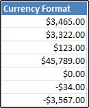
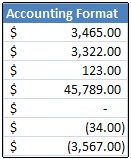
Both the Currency and Accounting formats are used to display monetary values. The difference between the two formats is explained in the following table.
| Format | Description | Example |
| Currency | When you apply the Currency format to a number, the currency symbol appears right next to the first digit in the cell. You can specify the number of decimal places that you want to use, whether you want to use a thousands separator, and how you want to display negative numbers. Tip: To quickly apply the Currency format, select the cell or range of cells that you want to format, and then press Ctrl+Shift+$. | |
| Format | Description | Example |
| Accounting | Like the Currency format, the Accounting format is used for monetary values. But, this format aligns the currency symbols and decimal points of numbers in a column. In addition, the Accounting format displays zeros as dashes and negative numbers in parentheses. Like the Currency format, you can specify how many decimal places you want and whether to use a thousands separator. You can't change the default display of negative numbers unless you create a custom number format. Tip: To quickly apply the Accounting format, select the cell or range of cells that you want to format. On the Home tab, in the Number group, click Accounting Number Format | |
Create a workbook template with specific currency formatting settings
If you often use currency formatting in your workbooks, you can save time by creating a workbook that includes specific currency formatting settings, and then saving that workbook as a template. You can then use this template to create other workbooks.
-
Create a workbook.
-
Select the worksheet or worksheets for which you want to change the default number formatting.
How to select worksheets
To select
Do this
A single sheet
Click the sheet tab.

If you don't see the tab that you want, click the tab scrolling buttons to display the tab, and then click the tab.

Two or more adjacent sheets
Click the tab for the first sheet. Then hold down Shift while you click the tab for the last sheet that you want to select.
Two or more nonadjacent sheets
Click the tab for the first sheet. Then hold down Ctrl while you click the tabs of the other sheets that you want to select.
All sheets in a workbook
Right-click a sheet tab, and then click Select All Sheets on the shortcut menu.
Tip When multiple worksheets are selected, [Group] appears in the title bar at the top of the worksheet. To cancel a selection of multiple worksheets in a workbook, click any unselected worksheet. If no unselected sheet is visible, right-click the tab of a selected sheet, and then click Ungroup Sheets.
-
Select the specific cells or columns you want to format, and then apply currency formatting to them.
Make any other customizations that you like to the workbook, and then do the following to save it as a template:
Save the workbook as a template
-
If you're saving a workbook to a template for the first time, start by setting the default personal templates location:
-
Click File, and then click Options.
-
Click Save, and then under Save workbooks, enter the path to the personal templates location in the Default personal templates location box.
This path is typically: C:\Users\Public Documents\My Templates.

-
Click OK.
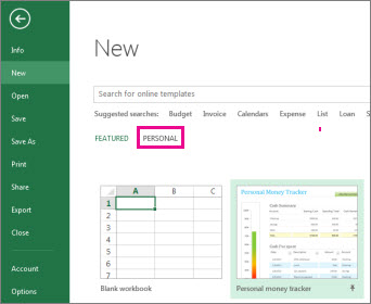
Once this option is set, all custom templates you save to the My Templates folder automatically appear under Personal on the New page (File > New).
-
-
Click File, and then click Export.
-
Under Export, click Change File Type.
-
In the Workbook File Types box, double-click Template.
-
In the File name box, type the name you want to use for the template.
-
Click Save, and then close the template.
Create a workbook based on the template
-
Click File, and then click New.
-
Click Personal.

-
Double-click the template you just created.
Excel creates a new workbook that is based on your template.


No comments:
Post a Comment