Sumproduct function

The SUMPRODUCT function returns the sum of the products of corresponding ranges or arrays. The default operation is multiplication, but addition, subtraction, and division are also possible.

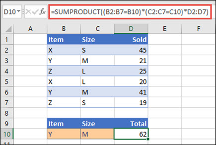
In this example, we'll use SUMPRODUCT to return the total sales for a given item and size:

SUMPRODUCT matches all instances of Item Y/Size M and sums them, so for this example 21 plus 41 equals 62.

Syntax

To use the default operation (multiplication):

=SUMPRODUCT(array1, [array2], [array3], ...)

The SUMPRODUCT function syntax has the following arguments:

Argument	Description
array1    Required	The first array argument whose components you want to multiply and then add.
[array2], [array3],...     Optional	Array arguments 2 to 255 whose components you want to multiply and then add.

To perform other arithmetic operations

Use SUMPRODUCT as usual, but replace the commas separating the array arguments with the arithmetic operators you want (*, /, +, -). After all the operations are performed, the results are summed as usual.

Note: If you use arithmetic operators, consider enclosing your array arguments in parentheses, and using parentheses to group the array arguments to control the order of arithmetic operations.

Remarks

• The array arguments must have the same dimensions. If they do not, SUMPRODUCT returns the #VALUE! error value. For example, =SUMPRODUCT(C2:C10,D2:D5) will return an error since the ranges aren't the same size.

• SUMPRODUCT treats non-numeric array entries as if they were zeros.

• For best performance, SUMPRODUCT should not be used with full column references. Consider =SUMPRODUCT(A:A,B:B), here the function will multiply the 1,048,576 cells in column A by the 1,048,576 cells in column B before adding them. 

Example 1

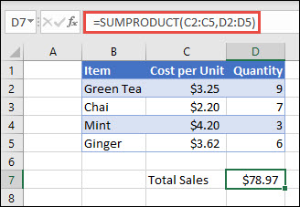
To create the formula using our sample list above, type =SUMPRODUCT(C2:C5,D2:D5) and press Enter. Each cell in column C is multiplied by its corresponding cell in the same row in column D, and the results are added up. The total amount for the groceries is $78.97.

To write a longer formula that gives you the same result, type =C2*D2+C3*D3+C4*D4+C5*D5 and press Enter. After pressing Enter, the result is the same: $78.97. Cell C2 is multiplied by D2, and its result is added to the result of cell C3 times cell D3 and so on.

Example 2

The following example uses SUMPRODUCT to return the total net sales by sales agent, where we have both total sales and expenses by agent. In this case, we're using an Excel table, which uses structured references instead of standard Excel ranges. Here you'll see that the Sales, Expenses, and Agent ranges are referenced by name.

The formula is: =SUMPRODUCT(((Table1[Sales])+(Table1[Expenses]))*(Table1[Agent]=B8)), and it returns the sum of all sales and expenses for the agent listed in cell B8.

Example 3

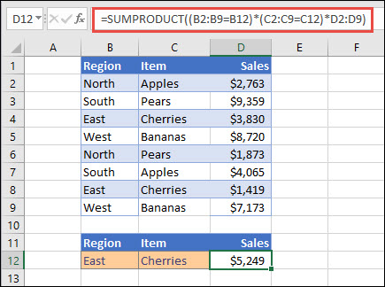
In this example, we want to return the total of a particular item sold by a given region. In this case, how many cherries did the East region sell?

Here, the formula is: =SUMPRODUCT((B2:B9=B12)*(C2:C9=C12)*D2:D9). It first multiplies the number of occurrences of East by the number of matching occurrences of cherries. Finally, it sums the values of the corresponding rows in the Sales column. To see how Excel calculates this, select the formula cell, then go to Formulas > Evaluate Formula > Evaluate.

Need more help?

You can always ask an expert in the Excel Tech Community, get support in the Answers community, or suggest a new feature or improvement on Excel User Voice.

See Also

Perform conditional calculations on ranges of cells

Sum based on multiple criteria with SUMIFS

Count based on multiple criteria with COUNTIFS

Average based on multiple criteria with AVERAGEIFS