Change the color of gridlines in a worksheet

By default, gridlines are displayed in worksheets using the color that is assigned to Automatic. To change the color of gridlines, you can use the following procedure.

1. Select the worksheets for which you want to change the gridline color.

2. Click File > Excel > Options.

3. In the Advanced category, under Display options for this worksheet, make sure that the Show gridlines check box is selected.

4. In the Gridline color box, click the color you want.

   

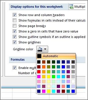
   Tip: To return gridlines to the default color, click Automatic.

Next steps

After you change the color of gridlines on a worksheet, you might want to take the following next steps:

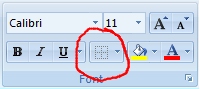
• Make gridlines more visible    To make the gridlines stand out on the screen, you can experiment with border and line styles. These settings are located on the Home tab, in the Font group.

  

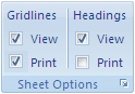
• Print gridlines    By default, Excel does not print gridlines on worksheets. If you want gridlines to appear on the printed page, select the worksheet or worksheets that you want to print. On the Page Layout tab, in the Sheet Options group, select the Print check box under Gridlines. To print, press CTRL+P.