Use slicers to filter PivotTable data
In earlier versions of Microsoft Excel, you can use report filters to filter data in a PivotTable report, but it is not easy to see the current filtering state when you filter on multiple items. In Microsoft Excel 2010, you have the option to use slicers to filter the data. Slicers provide buttons that you can click to filter PivotTable data. In addition to quick filtering, slicers also indicate the current filtering state, which makes it easy to understand what exactly is shown in a filtered PivotTable report.
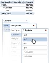
When you select an item, that item is included in the filter and the data for that item will be displayed in the report. For example, when you select Callahan in the Salespersons field, only data that includes Callahan in that field are displayed.
In this article
What are slicers?
Slicers are easy-to-use filtering components that contain a set of buttons that enable you to quickly filter the data in a PivotTable report, without the need to open drop-down lists to find the items that you want to filter.
When you use a regular PivotTable report filter to filter on multiple items, the filter indicates only that multiple items are filtered, and you have to open a drop-down list to find the filtering details. However, a slicer clearly labels the filter that is applied and provides details so that you can easily understand the data that is displayed in the filtered PivotTable report.
Slicers are typically associated with the PivotTable in which they are created. However, you can also create stand-alone slicers that are referenced from Online Analytical Processing (OLAP) Cube functions, or that can be associated with any PivotTable at a later time.
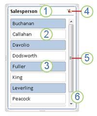
A slicer typically displays the following elements:
| | 1. A slicer header indicates the category of the items in the slicer. 2. A filtering button that is not selected indicates that the item is not included in the filter. 3. A filtering button that is selected indicates that the item is included in the filter. 4. A Clear Filter button removes the filter by selecting all items in the slicer. 5. A scroll bar enables scrolling when there are more items than are currently visible in the slicer. 6. Border moving and resizing controls allow you to change the size and location of the slicer. |
Using slicers
There are several ways to create slicers to filter your PivotTable data. In an existing PivotTable, you can:
-
Create a slicer that is associated with the PivotTable.
-
Create a copy of a slicer that is associated with the PivotTable.
-
Use an existing slicer that is associated with another PivotTable.
In addition to or instead of creating slicers in an existing PivotTable, you can also create a stand-alone slicer that can be referenced by Online Analytical Processing (OLAP) Cube functions or that you can associate with any PivotTable at a later time.
Because each slicer that you create is designed to filter on a specific PivotTable field, it is likely that you will create more than one slicer to filter a PivotTable report.
After you create a slicer, it appears on the worksheet alongside the PivotTable, in a layered display if you have more than one slicer. You can move a slicer to another location on the worksheet, and resize it as needed.

To filter the PivotTable data, you simply click one or more of the buttons in the slicer.
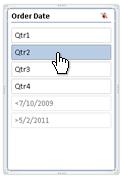
Formatting slicers for a consistent look
To create professional looking reports or simply to match the format of a slicer to the format of the associated PivotTable report, you can apply slicer styles for a consistent look. By applying one of the various predefined styles that are available for slicers, you can closely match the color theme that is applied to a PivotTable. For a custom look, you can even create your own slicer styles, just as you create custom PivotTable styles.
Sharing slicers between PivotTables
When you have many different PivotTables in one report, such as a Business Intelligence (BI) report that you are working with, it is likely that you will want to apply the same filter to some or all of those PivotTables. You can share a slicer that you created in one PivotTable with other PivotTables. No need to duplicate the filter for each PivotTable!
When you share a slicer, you are creating a connection to another PivotTable that contains the slicer that you want to use. Any changes that you make to a shared slicer are immediately reflected in all PivotTables that are connected to that slicer. For example, if you use a Country slicer in PivotTable1 to filter data for a specific country, PivotTable2 that also uses that slicer will display data for the same country.
Slicers that are connected to and used in more than one PivotTable are called shared slicers. Slicers that are used in one PivotTable only are called local slicers. A PivotTable can have both local and shared slicers.
Create a slicer in an existing PivotTable
-
Click anywhere in the PivotTable report for which you want to create a slicer.
This displays the PivotTable Tools, adding an Options and a Design tab.
-
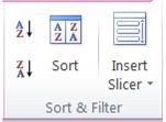
On the Options tab, in the Sort & Filter group, click Insert Slicer.
-
In the Insert Slicers dialog box, select the check box of the PivotTable fields for which you want to create a slicer.
-
Click OK.
A slicer is displayed for every field that you selected.
-
In each slicer, click the items on which you want to filter.
To select more than one item, hold down CTRL, and then click the items on which you want to filter.
Create a standalone slicer
-
On the Insert tab, in the Filter group, click Slicer.

-
In the Existing Connections dialog box, in the Show box, do one of the following:
-
To display all connections, click All Connections. This is selected by default.
-
To display only the recently used list of connections, click Connections in this Workbook.
This list is created from connections that you have already defined, that you have created by using the Select Data Source dialog box of the Data Connection Wizard, or that you have previously selected as a connection from this dialog box.
-
To display only the connections that are available on your computer, click Connection files on this computer.
This list is created from the My Data Sources folder that is usually stored in the My Documents folder.
-
To display only the connections that are available from a connection file that is accessed from the network, click Connection files on the Network.
This list is created from a Data Connection Library (DCL) on a Microsoft Office SharePoint Server 2007 or Microsoft SharePoint Server 2010 site. A DCL is a document library in a SharePoint Foundation site that contains a collection of Office Data Connection (ODC) files (.odc). Typically, a DCL is set up by a site administrator, who can also configure the SharePoint site to display ODC files from this DCL in the External Connections dialog box.
Tip If you do not see the connection that you want, you can create a connection. Click Browse for More, and then in the Select Data Source dialog box, click New Source to start the Data Connection Wizard so that you can select the data source that you want to connect to.
Note If you select a connection from the Connection files on the network or Connection files on this computer categories, the connection file is copied into the workbook as a new workbook connection, and is then used as the new connection information.
-
-
Under Select a Connection, click the connection that you want, and then click Open.
-
In the Insert Slicer dialog box, click the check box of the fields for which you want to create a slicer.
-
Click OK.
A slicer is created for every field that you selected.
Format a slicer
-
Click the slicer that you want to format.
This displays the Slicer Tools, adding an Options tab.
-
On the Options tab, in the Slicer Styles group, click the style that you want.
To see all available styles, click the More button
 .
.
Share a slicer by connecting to another PivotTable
You can share a slicer with another PivotTable by connecting it to that PivotTable. You can also insert a slicer from another PivotTable by connecting to that PivotTable.
Make a slicer available for use in another PivotTable
-
Click the slicer that you want to share in another PivotTable.
This displays the Slicer Tools, adding an Options tab.
-
On the Options tab, in the Slicer group, click PivotTable Connections.

-
In the PivotTable Connections dialog box, select the check box of the PivotTables in which you want the slicer to be available.
Use a slicer from another PivotTable
-
Create a connection to the PivotTable that contains the slicer that you want to share by doing the following:
-
On the Data tab, in the Get External Data group, click Existing Connections

-
In the Existing Connections dialog box, in the Show box, make sure that All Connections is selected.
Tip If you do not see the connection that you want, you can create a connection. Click Browse for More, and then in the Select Data Source dialog box, click New Source to start the Data Connection Wizard so that you can select the data source that you want to connect to.
-
Select the connection that you want, and then click Open.
-
In the Import Data dialog box, under Select how you want to view this data in your workbook, click PivotTable Report.
-
-
Click anywhere in the PivotTable report for which you want to insert a slicer from another PivotTable.
This displays the PivotTable Tools, adding an Options and a Design tab.
-
On the Options tab, in the Sort & Filter group, click the Insert Slicer arrow, and then click Slicer Connections.

-
In the Slicer Connections dialog box, select the check box of the slicers that you want to use.
-
Click OK.
-
In each slicer, click the items on which you want to filter.
To select more than one item, hold down CTRL, and then click the items that you want to filter.
Note All PivotTables that share the slicer will instantly display the same filtering state.
Disconnect or delete a slicer
If you no longer need a slicer, you can disconnect it from the PivotTable report, or you can delete it.
Disconnect a slicer
-
Click anywhere in the PivotTable report for which you want to disconnect a slicer.
This displays the PivotTable Tools, adding an Options and a Design tab.
-
On the Options tab, in the Sort & Filter group, click the Insert Slicer arrow, and then click Slicer Connections.

-
In the Slicer Connections dialog box, clear the check box of any PivotTable fields for which you want to disconnect a slicer.
Delete a slicer
Do one of the following:
-
Click the slicer, and then press DELETE.
-
Right-click the slicer, and then click Remove <Name of slicer>.
No comments:
Post a Comment