Perform Regression Analysis in Excel 2007
Microsoft Office Excel 2007 Inside Out
By Mark Dodge and Craig Stinson
Mark Dodge is a former senior technical writer for the Microsoft Office User Assistance group, and is the coauthor of four editions of Running Microsoft Excel. He was also a technical editor for over a dozen books on Microsoft applications. Mark has been honored with six awards from the Society for Technical Communication.
Craig Stinson has been an industry journalist since 1981, serving as a contributing editor of PC Magazine and author of the several editions of the best-selling Running Microsoft Windows®. In addition to being a coauthor on Running Microsoft Excel, he is the coauthor of Running Microsoft Windows NT® Workstation, Version 4. He has also written music reviews for such well-known publications as Billboard, the Boston Globe, and the Christian Science Monitor.
To learn more about other books on the 2007 Microsoft Office system, visit Microsoft Press.
In this article
Microsoft Office Excel 2007 provides a wide range of features that can help you analyze statistical data. This article focuses on how you can use regression analysis in Excel 2007 to analyze larger sets of data.
Understanding linear and exponential regression
Excel includes several array functions for performing linear regression (LINEST, TREND, FORECAST, SLOPE, and STEYX) and for performing exponential regression (LOGEST and GROWTH). You enter these functions as array formulas, and they produce array results. You can use each of these functions with one or several independent variables. The following list defines the different types of regression:
-
Linear regression Produces the slope of a line that best fits a single set of data. Based on a year's worth of sales figures, for example, linear regression can tell you the projected sales for March of the following year by giving you the slope and y-intercept (that is, the point where the line crosses the y-axis) of the line that best fits the sales data. By following the line forward in time, you can estimate future sales, if you can safely assume that growth will remain linear.
-
Exponential regression Produces an exponential curve that best fits a set of data that you suspect does not change linearly with time. For example, a series of measurements of population growth will nearly always be better represented by an exponential curve than by a line.
-
Multiple regression Is the analysis of more than one set of data, which often produces a more realistic projection. You can perform both linear and exponential multiple regression analyses. For example, suppose you want to project the appropriate price for a house in your area based on square footage, number of bathrooms, lot size, and age. Using a multiple regression formula, you can estimate a price, based on a database of information gathered from existing houses.
Regressing into the future?
The concept of regression might sound strange because the term is usually associated with movement backward, whereas in the world of statistics, regression is often used to predict the future. Simply put, regression is a statistical technique that finds a mathematical expression that best describes a set of data.
Often businesses try to predict the future using sales and percent-of-sales projections based on history. A simple percent-of-sales technique identifies assets and liabilities that vary along with sales, determines the proportion of each, and assigns them percentages. Although using percent-of-sales forecasting is often sufficient for slow or steady short-term growth, the technique loses accuracy as growth accelerates.
Regression analysis uses more sophisticated equations to analyze larger sets of data and translates them into coordinates on a line or curve. In the not-so-distant past, regression analysis was not widely used because of the large volume of calculations involved. Since spreadsheet applications, such as Excel, began offering built-in regression functions, the use of regression analysis has become more widespread.
Calculating linear regression
The equation y = mx + b algebraically describes a straight line for a set of data with one independent variable where x is the independent variable, y is the dependent variable, m represents the slope of the line, and b represents the y-intercept. If a line represents a number of independent variables in a multiple regression analysis to an expected result, the equation of the regression line takes the form
y=m 1 x 1 +m 2 x 2 +. . .+m n x n +b
in which y is the dependent variable, x1 through xn are n independent variables, m1 through mn are the coefficients of each independent variable, and b is a constant.
The LINEST function
The LINEST function uses this more general equation to return the values of m1 through mn and the value of b, given a known set of values for y and a known set of values for each independent variable. This function takes the form =LINEST(known_y's, known_x's, const, stats).
The known_y's argument is the set of y-values you already know. This argument can be a single column, a single row, or a rectangular range of cells. If known_y's is a single column, each column in the known_x's argument is considered an independent variable. Similarly, if known_y's is a single row, each row in the known_x's argument is considered an independent variable. If known_y's is a rectangular range, you can use only one independent variable; known_x's in this case should be a range of the same size and shape as known_y's. If you omit the known_x's argument, Excel uses the sequence 1, 2, 3, 4, and so on.
The const and stats arguments are optional. If either is included, it must be a logical constant—either TRUE or FALSE. (You can substitute 1 for TRUE and 0 for FALSE.) The default settings for const and stats are TRUE and FALSE, respectively. If you set const to FALSE, Excel forces b (the last term in the straight-line equation) to be 0. If you set stats to TRUE, the array returned by LINEST includes the following validation statistics:
| se1 through sen | Standard error values for each coefficient |
| seb | Standard error value for the constant b |
| r2 | Coefficient of determination |
| sey | Standard error value for y |
| F | F statistic |
| Df | Degrees of freedom |
| ssreg | Regression sum of squares |
| ssresid | Residual sum of squares |
Before creating a formula using LINEST, you must select a range large enough to hold the result array returned by the function. If you omit the stats argument (or set it explicitly to FALSE), the result array encompasses one cell for each of your independent variables and one cell for b. If you include the validation statistics, the result array looks like the following example. After selecting a range to contain the result array, type the function, and then press Ctrl+Shift+Enter to enter the function in each cell of the result array.
| mn | mn–1 | . . . | m2 | m1 | b |
| sen | sen–1 | . . . | se2 | se1 | seb |
| r2 | sey | ||||
| F | Df | ||||
| ssreg | ssresid |
Note that, with or without validation statistics, the coefficients and standard error values for your independent variables are returned in the opposite order from your input data. For example, if you have four independent variables organized in four columns, LINEST evaluates the leftmost column as x1, but it returns m1 in the fourth column of the result array.
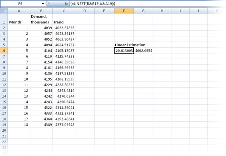
Figure 1 shows a simple example of the use of LINEST with one independent variable. The entries in column B of this worksheet represent monthly product demand for a small business. The numbers in column A represent the months in the period. Suppose you want to compute the slope and y-intercept of the regression line that best describes the relationship between the demand and the months. In other words, you want to describe the trend of the data. To do this, select the range F6:G6, type the formula =LINEST(B2:B19, A2:A19), and press Ctrl+Shift+Enter. The resulting number in cell F6 is 20.613, the slope of the regression line; the number in cell G6 is 4002.065, the y-intercept of the line.

The LINEST and LOGEST functions return only the y-axis coordinates used for calculating lines and curves. The difference between them is that LINEST projects a straight line and LOGEST projects an exponential curve. You must be careful to match the appropriate function to the analysis at hand. The LINEST function might be more appropriate for sales projections, and the LOGEST function might be more appropriate for statistical analyses or population trends.
Inside out a real (estate) regression application
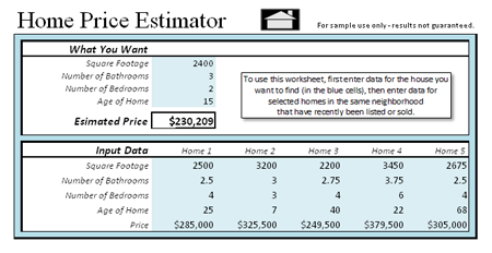
One often-used regression model is sometimes known as the Competitive Market Analysis (CMA). Realtors use CMAs to arrive at an estimated selling price for a home, based on historical sales data for comparable homes in the area. Here is a sample Excel-based version of this tool, called the Home Price Estimator:

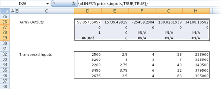
This application uses the LINEST function to analyze the statistics in the Input Data area and generate an array of results based on similar statistics in the What You Want area. The LINEST array is actually located in hidden rows below the visible area of the worksheet, as shown next. The first row of values in the LINEST data array is used by the Estimated Price formula to extrapolate an estimated value.

Usually in this workbook, row and column headings are hidden, rows 25 through 37 are hidden, worksheet protection is turned on, and cells are locked with entries allowed only in the designated input areas. Real estate tip: As the note on the worksheet implies, you can use listed home prices to arrive at an estimated price, but actual sale prices are more realistic, if you can get them.
The TREND function
LINEST returns a mathematical description of the straight line that best fits known data. TREND finds points that lie along that line and that fall into the unknown category. You can use the numbers returned by TREND to plot a trendline—a straight line that helps make sense of actual data. You can also use TREND to extrapolate, or make intelligent guesses about, future data based on the tendencies exhibited by known data. (Be careful. Although you can use TREND to plot the straight line that best fits the known data, TREND can't tell you whether that line is a good predictor of the future. Validation statistics returned by LINEST can help you make that assessment.) The TREND function takes the form =TREND(known_y's, known_x's, new_x's, const).
The first two arguments represent the known values of your dependent and independent variables. As in LINEST, the known_y's argument is a single column, a single row, or a rectangular range. The known_x's argument also follows the pattern described for LINEST. The third and fourth arguments are optional. If you omit new_x's, the TREND function considers new_x's to be identical to known_x's. If you include const, the value of that argument must be TRUE or FALSE (or 1 or 0). If const is TRUE, TREND forces b to be 0.
To calculate the trendline data points that best fit your known data, simply omit the third and fourth arguments from this function. The results array will be the same size as the known_x's range. In Figure 2, we used TREND to find the value of each point on the regression line that describes the data set from the example in Figure 1. To create these values, we selected the range C2:C19 and entered =TREND(B2:B19, A2:A19) as an array formula using Ctrl+Shift+Enter.
To extrapolate from existing data, you must supply a range for new_x's. You can supply as many or as few cells for new_x's as you want. The result array will be the same size as the new_x's range. In Figure 3 we used TREND to calculate demand for the 19th, 20th, and 21st months. To arrive at these values, we typed 19 through 21 in A21:A23, selected C21:C23, and entered =TREND(B2:B19, A2:A19, A21:A23) as an array formula by pressing Ctrl+Shift+Enter.
Calculating exponential regression
Unlike linear regression, which plots values along a straight line, exponential regression describes a curve by calculating the array of values needed to plot it. The equation that describes an exponential regression curve is as follows:
y = b * m1x1 * m2x2 * . . . * mnxn
If you have only one independent variable, the equation is as follows:
y = b * mx
The LOGEST function
The LOGEST function works like LINEST, except you use it to analyze data that is nonlinear, and it returns the coordinates of an exponential curve instead of a straight line. LOGEST returns coefficient values for each independent variable plus a value for the constant b. This function takes the form =LOGEST(known_y's, known_x's, const, stats).
LOGEST accepts the same arguments as the LINEST function and returns a result array in the same fashion. If you set the optional stats argument to TRUE, the function also returns validation statistics.
Note: The LINEST and LOGEST functions return only the y-axis coordinates used for calculating lines and curves. The difference between them is that LINEST projects a straight line and LOGEST projects an exponential curve. You must be careful to match the appropriate function to the analysis at hand. The LINEST function might be more appropriate for sales projections, and the LOGEST function might be more suited to applications such as statistical analyses or population trends.
The GROWTH function
Where the LOGEST function returns a mathematical description of the exponential regression curve that best fits a set of known data, the GROWTH function finds points that lie along that curve. The GROWTH function works like its linear counterpart, TREND, and takes the form =GROWTH(known_y's, known_x's, new_x's, const).

No comments:
Post a Comment