Filter data in a PivotTable
To focus on a smaller portion of a large amount of your PivotTable data for in-depth analysis, you can filter the data. There are several ways to do that. Start by inserting one or more slicers for a quick and effective way to filter your data. Slicers have buttons you can click to filter the data, and they stay visible with your data so you always know what fields are shown or hidden in the filtered PivotTable.
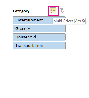
Tip: Now in Excel 2016, you can multi-select slicers by clicking the button on the label as shown above.
-
Click anywhere in the PivotTable to show the PivotTable Tools on the ribbon.

-
If you are using Excel 2016 or 2013, click Analyze > Insert Slicer.
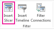
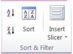
If you are using Excel 2010 or 2007, click Options > Insert Slicer > Insert Slicer.
-
In the Insert Slicers dialog box, check the boxes of the fields you want to create slicers for.
-
Click OK.
A slicer appears for each field you checked in the Insert Slicers dialog box.
-
In each slicer, click the items you want to show in the PivotTable.
To choose more than one item, hold down Ctrl, and then pick the items you want to show.
Tip: To change how the slicer looks, click the slicer to show the Slicer Tools on the ribbon, and then apply a slicer style or change settings on the Options tab.
Other ways to filter PivotTable data
Use any of the following filtering features instead of or in addition to using slicers to show the exact data you want to analyze.
Filter data manually
-
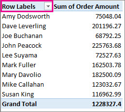
In the PivotTable, click the arrow
 on Row Labels or Column Labels.
-
In the list of row or column labels, uncheck the (Select All) box at the top of the list, and then check the boxes of the items you want to show in your PivotTable.
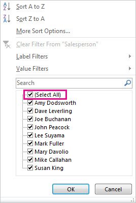
To see more items in the list, drag the handle in the bottom-right corner of the filter gallery to enlarge it.
-
Click OK.
The filtering arrow changes to this icon
 to indicate that a filter is applied. Click it to change or clear the filter by clicking Clear Filter From <Field Name>.
To remove all filtering at once, see the following:
-
In 2016 or 2013: Click anywhere in the PivotTable, and then click Analyze > Clear > Clear Filters.
-
In 2010 or 2007: click anywhere in the PivotTable, and then click Options > Clear > Clear Filters.

-
Use a report filter to filter items
Note: A report filter is labeled as Filters in PivotTable Fields pane in Excel 2016 and Excel 2013. See the screenshots below:
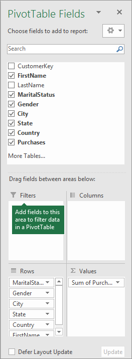 PivotTable Fields pane in Excel 2016 | 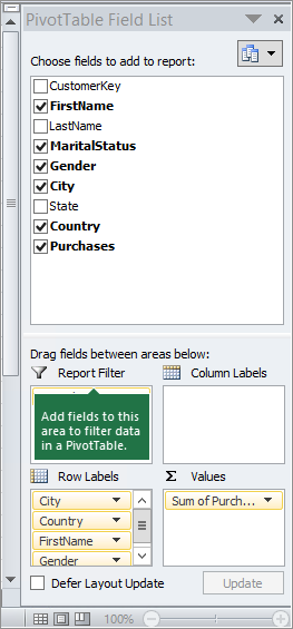 PivotTable Fields List pane in Excel 2010 |
By using a report filter, you can quickly display a different set of values in the PivotTable. Items you select in the filter are displayed in the PivotTable, and items that are not selected will be hidden. If you want to display filter pages (the set of values that match the selected report filter items) on separate worksheets, you can specify that option.
Add a report filter
-
Click anywhere inside the PivotTable.
The PivotTable Field List pane appears.
-
In the PivotTable Field List, click on the field in an area and select Move to Report Filter.
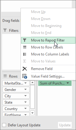
You can repeat this step to create more than one report filter. Report filters are displayed above the PivotTable for easy access.
-
To change the order of the fields, in the Report Filter area, drag the fields to the position that you want. The order of the report filters will be reflected in the PivotTable.
Display report filters in rows or columns
-
Click the PivotTable or the associated PivotTable of a PivotChart.
-
Right-click anywhere in the PivotTable, and then click PivotTable Options.
-
In the Layout & Format tab, specify these options:
-
Under Layout, in the Display fields in report filter area list box, do one of the following:
-
To display report filters in columns from left to right, select Over, Then Down.
-
To display report filters in rows from top to bottom, select Down, Then Over.
-
-
In the Report filter fields per column or Report filter fields per row box, type or select the number of fields to display before taking up another column or row based on the setting of Display fields in report filter area.
Select items in the report filter
-
In the PivotTable, click the dropdown arrow next to the report filter.

-
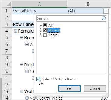
To display a check box for all items so that you can clear or select them as needed, select the Select Multiple Items check box.
-
You can now select the checkboxes next to the items that you want to display in the report. To select all items, click the checkbox next to (All).
-
Click OK. At least one check box should be selected for this button to be enabled.
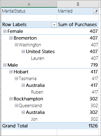
The report filter now displays the filtered items.
Note: If you are using an OLAP data source is Microsoft SQL Server Analysis Services (version 2005 or later), you can only select a calculated member if it is a single item, you cannot select multiple items when one or more of those items are calculated members.
Display report filter pages on separate worksheets
-
Click anywhere in the PivotTable (or the associated PivotTable of a PivotChart ) that has one or more report filters.
-
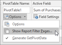
If you are using Excel 2016 or 2013, click the Analyze tab, in the PivotTable group, click the arrow next to Options, and then click Show Report Filter Pages.
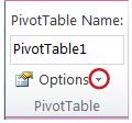
If you are using Excel 2010 or 2007, click the Options tab, in the PivotTable group, click the arrow next to Options, and then click Show Report Filter Pages.
-
In the Show Report Filter Pages dialog box, select a report filter field, and then click OK.
Show specific text, values, or dates only
-
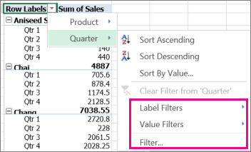
In the PivotTable, right-click any text, value, or date field label, and then click Label Filters, Value Filters, or Date Filters.
-
Click the comparison operator command you want to use.
For example, to filter by text that begins with a specific character, select Begins With, or to filter by text that has specific characters anywhere in the text, select Contains.
Note: Label Filters is not available when row label or column label fields don't have text-based labels.
-
Do one of the following:
-
In the Label Filter <Field name> dialog box, enter the text you want to filter by.
For example, to filter by text that begins with the letter "J", enter J, or to filter by text that has "bell" anywhere in the text, enter bell.
If the PivotTable is based on a non-OLAP data source, you can use the following wild card characters to find data that have specific characters.
-
| Use | To find |
| ? (question mark) | Any single character |
| * (asterisk) | Any number of characters |
| ~ (tilde) followed by ?, *, or ~ | A question mark, asterisk, or tilde |
-
In the Value Filter <Field name> dialog box, enter the values you want to filter by.
-
In the Date Filter <Field name> dialog box, enter the dates you want to filter by.
If the PivotTable is based on an OLAP data source, date filters require the OLAP cube field hierarchy data type of time. If a date is entered as text in a text field, the date filter won't be available.
Tip: To remove a label, date, or value filter, click the arrow  in the row or column label, click Label Filter, Date Filter, or Value Filter, and then click Clear Filter.
Show the top or bottom 10 items
You can also apply filters to show the top or bottom 10 values or data that meets the certain conditions.
-
In the PivotTable, click the arrow
 on Row Labels or Column Labels, click Value Filters, and then click Top 10.
 -
In the Top 10 Filter <Field Name> dialog box, do the following.
-
In the first box, click Top or Bottom.
-
In the second box, enter a number.
-
In the third box, pick the option you want to filter by.
-
To filter by number of items, pick Items.
-
To filter by percentage, pick Percent.
-
To filter by sum, pick Sum.
-
-
In the fourth box, pick the field you want.
-
Filter by selection to display or hide selected items only
-
In the PivotTable, select one or more items in the field that you want to filter by selection.
You can make a discontinuous selection by holding down CTRL when you select items.
-
Right-click an item in the selection, and then click Filter.
-
Do one of the following:
-
To display the selected items, click Keep Only Selected Items.
-
To hide the selected items, click Hide Selected Items.
Tip: You can display hidden items again by removing the filter. Right-click another item in the same field, click Filter, and then click Clear Filter.
-
Turn filtering options on or off
If you want to apply multiple filters per field, or if you don't want to show Filter buttons in your PivotTable, here's how you can turn these and other filtering options on or off:
-
Click anywhere in the PivotTable to show the PivotTable Tools on the ribbon.

-
On the Options tab, in the PivotTable group, click Options.

-
In the PivotTable Options dialog box, click the Totals & Filters tab.
-
Under Filters, do any of the following:
-
To use or not use multiple filters per field, check or uncheck the Allow multiple filters per field box.
-
To include or exclude filtered items in totals, check or uncheck the Include filtered items in totals box, and then check or uncheck the Mark totals with * box. If checked, an asterisk (*) indicator appears in totals outside of fields that have visual totals turned off. This option is available only in PivotTables that are connected to an OLAP data source that supports the MDX expression language. It affects all fields in the PivotTable.
-
To include or exclude filtered items in totals for named sets, check or uncheck the Include filtered items in set totals box. This option is available only in PivotTables that are connected to an OLAP data source.
-
To include or exclude filtered items in subtotals, select or clear the Subtotal filtered page items box.
-
-
To show or hide field captions and filter drop downs, click the Display tab, and then check or uncheck the Display field captions and filter drop downs check box.
-
Click anywhere in the PivotTable to show the PivotTable tabs (PivotTable Analyze and Design) on the ribbon.
-
Click PivotTable Analyze > Insert Slicer.
-
In the Insert Slicers dialog box, check the boxes of the fields you want to create slicers for.
-
Click OK.
A slicer appears for each field you checked in the Insert Slicers dialog box.
-
In each slicer, click the items you want to show in the PivotTable.
Tip: To change how the slicer looks, click the slicer to show the Slicer tab on the ribbon. You can apply a slicer style or change settings using the various tab options.
Other ways to filter PivotTable data
Use any of the following filtering features instead of or in addition to using slicers to show the exact data you want to analyze.
Use a report filter to filter items
Show the top or bottom 10 items
Filter data manually
-
In the PivotTable, click the arrow
 on Row Labels or Column Labels.
 -
In the list of row or column labels, uncheck the (Select All) box at the top of the list, and then check the boxes of the items you want to show in your PivotTable.
-
The filtering arrow changes to this icon
 to indicate that a filter is applied. Click it to change or clear the filter by clicking Clear Filter From <Field Name>.
To remove all filtering at once, click PivotTable Analyze tab > Clear > Clear Filters.
Use a report filter to filter items
By using a report filter, you can quickly display a different set of values in the PivotTable. Items you select in the filter are displayed in the PivotTable, and items that are not selected will be hidden. If you want to display filter pages (the set of values that match the selected report filter items) on separate worksheets, you can specify that option.
Add a report filter
-
Click anywhere inside the PivotTable.
The PivotTable Fields pane appears.
-
In the PivotTable Field List, click on the field in an area and select Move to Report Filter.
You can repeat this step to create more than one report filter. Report filters are displayed above the PivotTable for easy access.
-
To change the order of the fields, in the Filters area, you can either drag the fields to the position that you want, or double-click on a field and select Move Up or Move Down. The order of the report filters will be reflected accordingly in the PivotTable.
Display report filters in rows or columns
-
Click the PivotTable or the associated PivotTable of a PivotChart.
-
Right-click anywhere in the PivotTable, and then click PivotTable Options.
-
In the Layout tab, specify these options:
-
In Report Filter area, in the Arrange fields list box, do one of the following:
-
To display report filters in rows from top to bottom, select Down, Then Over.
-
To display report filters in columns from left to right, select Over, Then Down.
-
-
In the Filter fields per column box, type or select the number of fields to display before taking up another column or row (based on the setting of Arrange fields you specified in the previous step).
-
Select items in the report filter
-
In the PivotTable, click the dropdown arrow next to the report filter.
-
Select the checkboxes next to the items that you want to display in the report. To select all items, click the checkbox next to (Select All).
The report filter now displays the filtered items.
Display report filter pages on separate worksheets
-
Click anywhere in the PivotTable (or the associated PivotTable of a PivotChart ) that has one or more report filters.
-
Click PivotTable Analyze (on the ribbon) > Options > Show Report Filter Pages.
-
In the Show Report Filter Pages dialog box, select a report filter field, and then click OK.
Show the top or bottom 10 items
You can also apply filters to show the top or bottom 10 values or data that meets the certain conditions.
-
In the PivotTable, click the arrow
 next to Row Labels or Column Labels.
 -
Right-click an item in the selection, and then click Filter > Top 10 or Bottom 10.
-
In the first box, enter a number
-
In the second box, pick the option you want to filter by. The following options are available:
-
To filter by number of items, pick Items.
-
To filter by percentage, pick Percentage.
-
To filter by sum, pick Sum.
-
-
In the search box, you can optionally search for a particular value.
Filter by selection to display or hide selected items only
-
In the PivotTable, select one or more items in the field that you want to filter by selection.
-
Right-click an item in the selection, and then click Filter.
-
Do one of the following:
-
To display the selected items, click Keep Only Selected Items.
-
To hide the selected items, click Hide Selected Items.
Tip: You can display hidden items again by removing the filter. Right-click another item in the same field, click Filter, and then click Clear Filter.
-
Turn filtering options on or off
If you want to apply multiple filters per field, or if you don't want to show Filter buttons in your PivotTable, here's how you can turn these and other filtering options on or off:
-
Click anywhere in the PivotTable to show the PivotTable tabs on the ribbon.
-
On the PivotTable Analyze tab, click Options.
-
In the PivotTable Options dialog box, click the Layout tab.
-
In the Layout area, check or uncheck the Allow multiple filters per field box depending on what you need.
-
Click the Display tab, and then check or uncheck the Field captions and filters check box, to show or hide field captions and filter drop downs
-
You can view and interact with PivotTables in Excel Online, which includes some manual filtering and using slicers that were created in the Excel desktop application to filter your data. You won't be able to create new slicers in Excel Online.
To filter your PivotTable data, do one of the following:
-
To apply a manual filter, click the arrow on Row Labels or Column Labels, and then pick the filtering options you want.
-
If your PivotTable has slicers, just click the items you want to show in each slicer.

If you have the Excel desktop application, you can use the Open in Excel button to open the workbook and apply additional filters or create new slicers for your PivotTable data there. Here's how:
Click Open in Excel and filter your data in the PivotTable.

For news about the latest Excel Online updates, visit the Microsoft Excel blog.
For the full suite of Office applications and services, try or buy it at Office.com.
No comments:
Post a Comment