Tutorial create map based power view reports

Abstract:    This is the third tutorial in a series. In the first tutorial, Import Data into Excel 2013, and Create a Data Model, you created an Excel workbook from scratch using data imported from multiple sources, and its Data Model was created automatically by Excel. The second tutorial,Extend Data Model relationships using Excel 2013, Power Pivot, and DAX, you learned how to extend the Data Model and created hierarchies within the data.

In this tutorial, you use that extended Data Model to build compelling reports that include multiple visualizations using Power View.

The sections in this tutorial are the following:

• Create a Power View report

• Create calculated fields for Power View and PivotTables

• Set field defaults, table behaviors, and data categories

• Checkpoint and Quiz

At the end of this tutorial is a quiz you can take to test your learning.

This series uses data describing Olympic Medals, hosting countries, and various Olympic sporting events. The tutorials in this series are the following:

1. Import Data into Excel 2013, and Create a Data Model

2. Extend Data Model relationships using Excel 2013, Power Pivot, and DAX

3. Create Map-based Power View Reports

4. Incorporate Internet Data, and Set Power View Report Defaults

5. Power Pivot Help

6. Create Amazing Power View Reports - Part 2

We suggest you go through them in order.

These tutorials use Excel 2013 with Power Pivot enabled. For guidance on enabling Power Pivot, click here.

Create a Power View report

In the previous tutorials, you created an Excel workbook with a PivotTable containing data about Olympic medals and events. If you didn't complete the previous tutorial, you can download the workbook from the end of the previous tutorial from here.

In this section, you create a Power View report to visually represent the Olympics data.

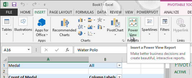
1. In Excel, click INSERT > Reports > Power View Reports.
   
   

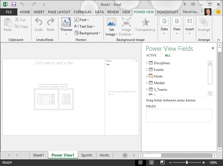
2. A blank Power View report appears as a sheet in the workbook.
   
   
    

3. In the Power View Fields area, click the arrow beside Hosts to expand it, and click City.

4. Expand the Medals table, and click Sport. With this, Power View lists the Sport beside the city, as shown in the following screen.
   

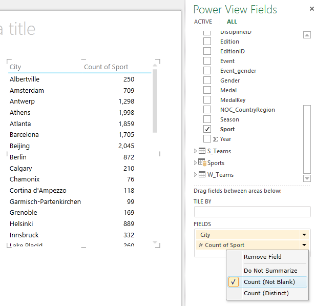
5. In the FIELDS area of Power View Fields, click the arrow next to Sport and select Count (Not Blank). Now Power View is counting the sports, rather than listing them, as shown in the following screen.
   
   

6. On the ribbon, select DESIGN > Switch Visualization > Map. The DESIGN tab is only available if the Power View table is selected. You may get a warning about enabling external content when you switch to the Map visualization.

7. A map replaces the table as the visualization. On the map, blue circles of varying size indicate the number of different sport events held at each Olympic Host location. But it might be more interesting to see which were summer events, and which were winter.

8. To make the most use of the report area, let's collapse the Filters area. Click the arrow in the upper right corner of the Filters area.

9. In Power View Fields, expand Medals. Drag the Season field down to the COLOR area. That's better: the map now displays blue bubbles for summer sports, and red bubbles for winter sports, as shown in the following screen. You can resize the visualization by dragging any of its corners.
   
   

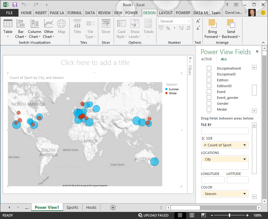
Now you have a Power View report that visualizes the number of sporting events in various locations, using a map, color-coded based on season. And it just took a few clicks.

Create calculated fields for Power View and PivotTables

Power View uses the underlying Data Model to create visualizations. With Power Pivot and DAX, you can extend the Data Model by creating custom formulas, then create reports based on those formulas and calculations in PivotTables and in Power View.

Create a calculated field in Power Pivot

1. In Excel, click Power Pivot > Data Model > Manage to display the Power Pivot window.

2. Select the Medals table. Make sure the Calculation Area is displayed. The Calculation Area is found below the table data, and is used for creating, editing, and managing calculated fields. To view the Calculation Area, select Home > View > Calculation Area, as shown in the following screen.
   
   

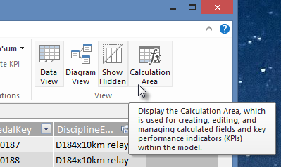
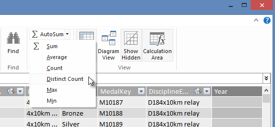
3. Let's calculate the number of Olympic editions. In the Calculation Area, select the cell directly below the Edition column. From the ribbon, select AutoSum > Distinct Count, as shown in the following screen.
   
   

4. Power Pivot creates a DAX expression for the active cell in the Calculation Area. In this case, Power Pivot automatically created the following DAX formula:
   
   Distinct Count of Edition:=DISTINCTCOUNT([Edition])
   
   Additional calculations in AutoSum are just as easy, such as Sum, Average, Min, Max, and others.

5. Save the Excel workbook. The Data Model is updated with the new calculated field. When you return to the Power View tab in Excel, a warning lets you know the Data Model has been updated, as shown in the following screen.
   
   

We'll use this Distinct Count of Edition calculated field later on in the tutorials.

Create a calculated field using DAX in Power Pivot

The AutoSum calculation is useful, but there are times when more customized calculations are required. You can create DAX formulas in the Calculation Area, just like you create formulas in Excel. Let's create a DAX formula and then see how it appears in our Data Model, and as a result, is available in our PivotTable and in Power View.

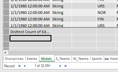
1. Open the Power Pivot window. In the Calculation Area, select the cell directly below the AutoSum calculation you completed in the previous section, as shown in the following screen.
   
   

2. Let's calculate the percentage of all medals. In the formula bar, type the following DAX formula. IntelliSense provides available commands based on what you type, and you can press Tab to select the highlighted IntelliSense option.
   
   Percentage of All Medals:=[Count of Medal]/CALCULATE([Count of Medal],ALL(Medals))

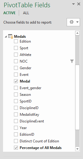
3. When you switch back to the Excel window, Excel lets you know the Data Model has been updated. In Excel, select the PivotTable in Sheet1. In PivotTable Fields, expand the Medals table. At the bottom of the fields list are the two calculated fields we just created, as shown in the following screen. Select Percentage of All Medals.
   
   

4. In the PivotTable, the Percentage of All Medals field appears after Count of Medal. It's not formatted as a percentage, so select those fields (you can select them all at once, by hovering over the top of one of the Percentage of All Medals field, until the cursor becomes a down arrow, and then clicking). Once they're selected, click HOME > Number > Percentage. In the same section of the ribbon, adjust the number of decimal places to two. Your pivot table looks like the following screen.
   
   

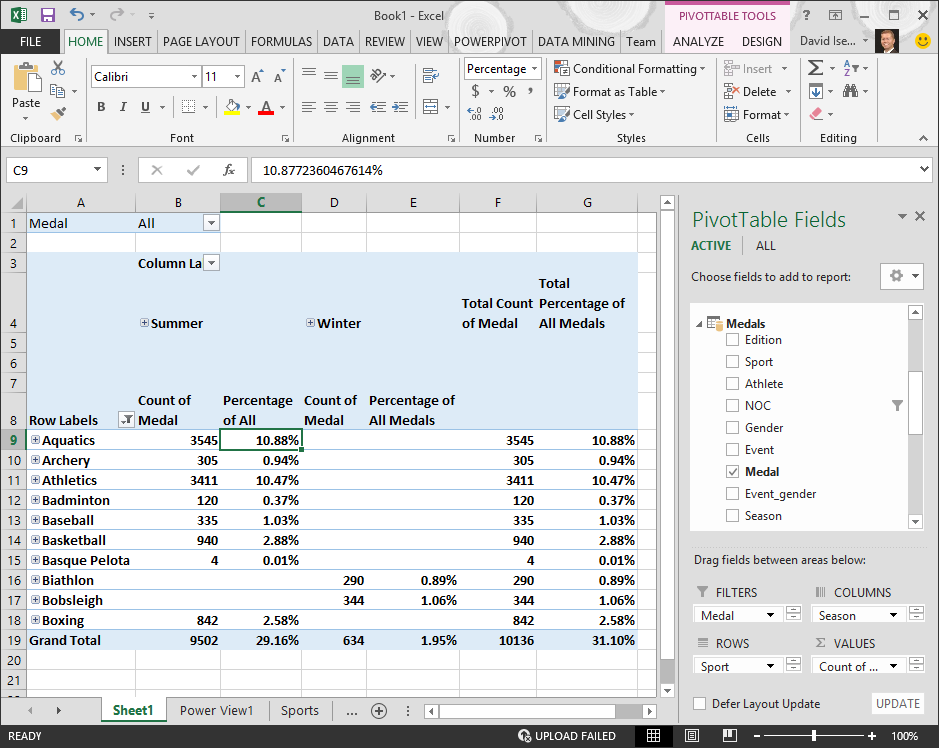
In a previous tutorial, we filtered the Sports field to only the first ten, alphabetically, which is why we only see Aquatics through Boxing, and why the percentage in the Grand Total is 29.16%, rather than 100%. What this does tell us, of course, is that these first ten sports account for 29.16% of all medals awarded in the Summer games. We also can see that Aquatics accounted for 10.88% of all medals.

Since the Percentage of All Medals field is in the Data Model, it's also available in Power View.

You can also create calculated fields from the Power Pivot tab while in Power View. Whether you create a calculated field in Power Pivot or while in Power View, the result is the same: the Data Model is updated to include the calculated field, and makes it available to all client tools.

Set field defaults, table behaviors, and data categories

Another way to streamline report creation in Power View is by setting a default field set. When you set a default field set for a table, you can simply click that table in Power View, and the default set of fields is automatically added to a new report.

In this section, you set defaults for your workbook that will save you time when creating reports.

Create the Default Field Set for a table

1. The Power Pivot window should still be available. If not, click Power Pivot > Data Model> Manage. In Power Pivot, select Home > View > Data View to make sure Data View is selected. Select the Medals table.

2. On the Advanced tab, click Reporting Properties > Default Field Set. A window appears that lets you specify default fields for tables created using client tools such as Power View.

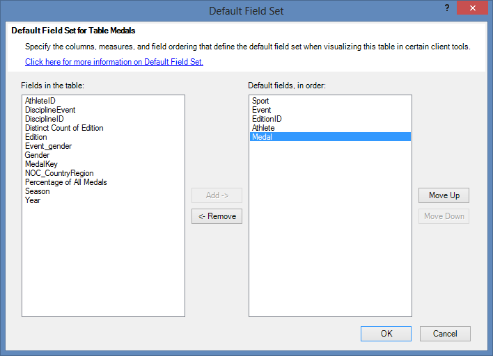
3. Select Sport, Event, EditionID, Athlete, and Medal in the left pane, and click Add -> to make them the default fields. Make sure they appear in the right pane, Default fields, in the order they were listed. The Default Field Set window looks like the following screen.
   
   

4. Click OK to save the default field set for the Medals table.

5. To see how this works, switch to the Power View sheet in Excel.

6. Click anywhere on the blank report canvas, to make sure you don't have an existing visualization selected. Your Power View sheet currently only has one visualization, which is the map you created earlier.

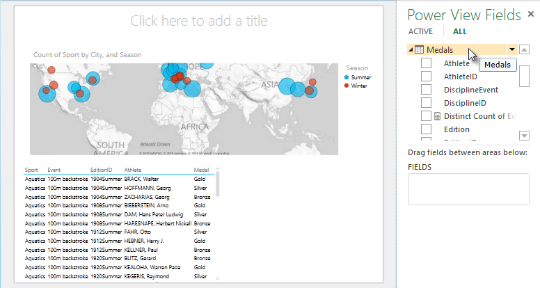
7. In the Power View Fields list, click the Medals table name. Power View creates a table and automatically adds the five default fields from the Medals table, in the order you specified, as shown in the following screen. If you accidentally click on the triangle beside Medals, the table simply expands, rather than adding a new table with default fields.
   
   

Set Table Behavior

You can also set the default table behavior, which Power View uses to automatically create report labels for the table. This becomes useful when you create visualizations from the same table, perhaps for many different reports. We use default table behavior in the next few steps, so let's set it now.

1. Back in Power Pivot, with the Medals table selected, select Advanced > Reporting Properties > Table Behavior. A window appears where you can specify table behavior.

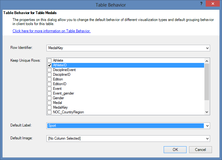
2. In the Table Behavior window, the Row Identifier is the column that contains only unique keys and no blank values. This is often the table's primary key, but doesn't have to be. You have to select a Row Identifier before making other selections in the window. Select MedalKey as the Row Identifier.

3. In the Keep Unique Rows section, select AthleteID. Fields you select here have row values that should be unique, and should not be aggregated when creating Pivot Tables or Power View reports.
   
   Note: If you have trouble with reports that don't aggregate how you want them to, ensure the field you want to aggregate is not selected in the Keep Unique Rows fields.

4. For Default Label, select a key that should be used as a default report label. Select Sport.

5. For Default Image, leave the selection as [No Column Selected], since you haven't added images yet. The Table Behavior window looks like the following screen.
   
   

6. Click OK. On the Power View sheet in Excel, select the table you created in the previous steps. From the ribbon, select DESIGN > Table > Card. The table you created changes into a collection of Cards; the data is the same, but the visualization of the data has changed. The table now looks like the following screen.
   

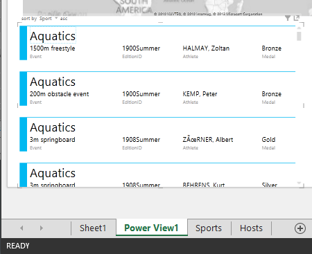
Notice that the Sport field is larger than the rest, and appears as a heading for each card. That's because you set Sport as the Default Label in the Table Behavior window when you were in Power Pivot.

Set Data Categories for fields

In order for Power View to dynamically create reports based on underlying data, such as location, fields that contain such data must be properly categorized. For the Olympics data, let's specify the categories for a few fields.

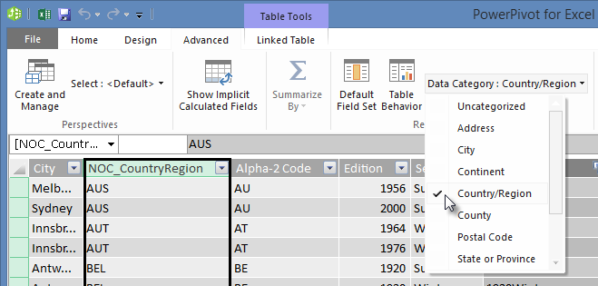
1. In Power Pivot, select Hosts. Select the NOC_CountryRegion field. From Advanced > Reporting Properties > Data Category: click the arrow and select Country/Region from the list of available data categories, as shown in the following screen.
   
   

2. In Medals, select the NOC_CountryRegion column. Again, change the Data Category to Country/Region.

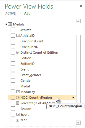
3. Return to Excel, and select the Power View sheet. Expand the Medals table in Power View Fields, and notice that the NOC_CountryRegion field now has a small globe icon beside it. The globe indicates that NOC_CountryRegion contains a geographic location, as shown in the following screen.
   
   

We'll use that geographic location in an upcoming tutorial. It's time to save your work, review what you've learned, and then get ready to dive into the next tutorial.

Checkpoint and Quiz

Review what you learned

In this tutorial you learned how to create a map-based Power View visualization, then created calculated fields to extend your Data Model, and analyze the data in a different way. You also learned how to create default field sets for a table, which streamlined creating a new Power View table pre-populated with the default set of fields. You also learned how to define default table behavior, so the ordering and labeling of new tables was fast and consistent.

In the next tutorial in this series, you build on what you learned here. There's a lot of data out there, and in the next tutorial, you add Internet data into your Data Model, and bring in images so that your Power View reports can really shine.

Here's a link to the next tutorial:

Tutorial: Incorporate Internet Data, and Set Power View Report Defaults

QUIZ

Want to see how well you remember what you learned? Here's your chance. The following quiz highlights features, capabilities, or requirements you learned about in this tutorial. At the bottom of the page, you'll find the answers. Good luck!

Question 1: Where does Power View get its data to create Power View reports?

A: Only from worksheets included in Excel.

B: Only from the Data Model.

C: Only from data imported from external sources.

D: From the Data Model, and from any data that exists in the worksheets in Excel.

Question 2: Which of the following is true about a default field set?

A: You can only create one default field set for the entire Data Model.

B: In Power View, clicking the table name in Power View Fields creates a table visualization that is automatically populated with the its default field set.

C: If you create a default field set for a table, all other fields in that table are disabled.

D: All of the above

Question 3: Which of the following is true about Calculated Fields?

A: When you create them in Power Pivot, they appear in Power View as fields available in the table in which they were created.

B: If you create them in the Calculation Area of Power Pivot, they are hidden from all client tools.

C: When you create them in Power Pivot, they each appear as individual tables in all client tools.

D: Both A and B.

Question 4: In the Default Behavior Table window, if you select a field in Keep Unique Rows, which of the following is correct?

A: You must explicitly select "Sum this field" from Power View Fields in order to aggregate the field.

B: The field is always aggregated in Power View or PivotTables.

C: The field is never aggregated in Power View or PivotTables.

D: Selecting Keep Unique Rows has no effect on the behavior of the field in Power View or PivotTables.

Quiz an swers

1. Correct answer: B

2. Correct answer: B

3. Correct answer: A

4. Correct answer: C

Notes: 

• Data and images in this tutorial series are based on the following:

• Olympics Dataset from Guardian News & Media Ltd.

• Flag images from CIA Factbook (cia.gov)

• Population data from The World Bank (worldbank.org)

• Olympic Sport Pictograms by Thadius856 and Parutakupiu