Sometimes duplicate data is useful, sometimes it just makes it harder to understand your data. Use conditional formatting to find and highlight duplicate data. That way you can review the duplicates and decide if you want to remove them.
-
Select the cells you want to check for duplicates.
Note: Excel can't highlight duplicates in the Values area of a PivotTable report.
-
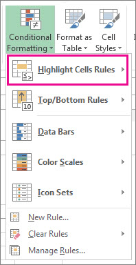
Click Home > Conditional Formatting > Highlight Cells Rules > Duplicate Values.

-
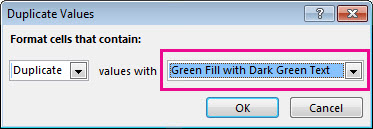
In the box next to values with, pick the formatting you want to apply to the duplicate values, and then click OK.

Remove duplicate values
When you use the Remove Duplicates feature, the duplicate data will be permanently deleted. Before you delete the duplicates, it's a good idea to copy the original data to another worksheet so you don't accidentally lose any information.
-
Select the range of cells that has duplicate values you want to remove.
Tip: Remove any outlines or subtotals from your data before trying to remove duplicates.
-
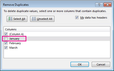
Click Data > Remove Duplicates, and then Under Columns, check or uncheck the columns where you want to remove the duplicates.

For example, in this worksheet, the January column has price information I want to keep.

So, I unchecked January in the Remove Duplicates box.

-
Click OK.
No comments:
Post a Comment