Create power query formulas in excel

Note: This article has done its job, and will be retiring soon. To prevent "Page not found" woes, we're removing links we know about. If you've created links to this page, please remove them, and together we'll keep the web connected.

Note:  Power Query is known as Get & Transform in Excel 2016. Information provided here applies to both. To learn more, see Get & Transform in Excel 2016.

To create Power Query formulas in Excel, you can use the Query Editor formula bar, or the Advanced Editor. The Query Editor is a tool included with Power Query that lets you create data queries and formulas in Power Query. The language used to create those formulas is the Power Query Formula Language. There are many Power Query formulas you can use to discover, combine and refine data. To learn more about the full range of Power Query formulas, see Power Query formula categories.

Let's create a simple formula, and then create an advanced formula.

• Create a simple formula

• Create an advanced formula

Create a simple formula

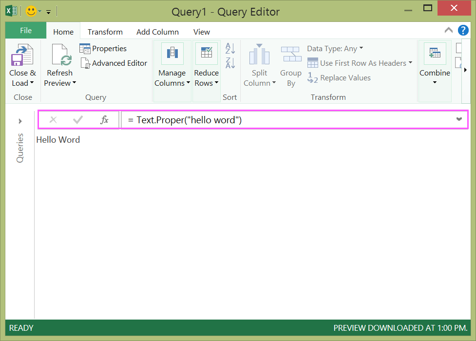
For a simple formula example, let's convert a text value to proper case using the Text.Proper() formula.

1. In the POWER QUERY ribbon tab, choose From Other Sources > Blank Query.

   

2. In the Query Editor formula bar, type = Text.Proper("text value"), and press Enter or choose the Enter icon.

3. Power Query shows you the results in the formula results pane.

4. To see the result in an Excel worksheet, choose Close & Load.

The result will look like this in a worksheet:

You can also create advanced query formulas in the Query Editor.

Create an advanced formula

For an advanced formula example, let's convert the text in a column to proper case using a combination of formulas. You can use the Power Query Formula Language to combine multiple formulas into query steps that have a data set result. The result can be imported into an Excel worksheet.

Note: This topic is an introduction to advanced Power Query formulas. To learn more about Power Query formulas, see Learn about Power Query formulas.

For example, let's assume you have an Excel table with product names you want to convert to proper case.

The original table looks like this:

And, you want the resulting table to look like this:

Let's go through the query formula steps to change the original table so that the values in the ProductName column are proper case.

Advanced query using Advanced Editor example

To clean up the original table, you use the Advanced Editor to create query formula steps. Let's build each query formula step to show how to create an advanced query. The complete query formula steps are listed below. When you create an advanced query, you follow this process:

• Create a series of query formula steps that start with the let statement. Please note that the Power Query Formula Language is case sensitive.

• Each query formula step builds upon a previous step by referring to a step by name.

• Output a query formula step using the in statement. Generally, the last query step is used as the in final data set result.

Step 1 – Open Advanced Editor

1. In the POWER QUERY ribbon tab, choose From Other Sources > Blank Query.

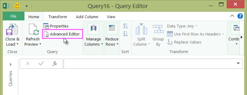
2. In Query Editor, choose Advanced Editor.

   

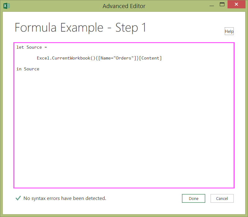
3. You will see the Advanced Editor.

   

Step 2 – Define the original source

In the Advanced Editor:

1. Use a let statement that assigns Source = Excel.CurrentWorkbook() formula. This will use an Excel table as the data source. For more information about the Excel.CurrentWorkbook() formula, see Excel.CurrentWorkbook.

2. Assign Source to the in result.

   let Source =  Excel.CurrentWorkbook(){[Name="Orders"]}[Content]  in Source

3. Your advanced query will look like this in the Advanced Editor.

   

4. To see the results in a worksheet:

   1. Click Done.

   2. In the Query Editor ribbon, click Close & Load.

The result looks like this in a worksheet:

Step 3 – Promote the first row to headers

To convert the values in the ProductName column to proper text, you first need to promote the first row to become the column headers. You do this in the Advanced Editor:

1. Add a #"First Row as Header" = Table.PromoteHeaders() formula to your query formula steps and refer to Source as the data source. For more information about the Table.PromoteHeaders() formula, see Table.PromoteHeaders.

2. Assign #"First Row as Header" to the in result.

   let      Source = Excel.CurrentWorkbook(){[Name="Orders"]}[Content],      #"First Row as Header" = Table.PromoteHeaders(Source)  in      #"First Row as Header"

The result looks like this in a worksheet:

Step 4 – Change each value in a column to proper case

To convert each ProductName column value to proper text, you use Table.TransformColumns() and refer to the "First Row as Header" query formula step. You do this in the Advanced Editor:

1. Add a #"Capitalized Each Word" = Table.TransformColumns() formula to your query formula steps and refer to #"First Row as Header" as the data source. For more information about the Table.TransformColumns() formula, see Table.TransformColumns.

2. Assign #"Capitalized Each Word" to the in result.

let      Source = Excel.CurrentWorkbook(){[Name="Orders"]}[Content],      #"First Row as Header" = Table.PromoteHeaders(Source),      #"Capitalized Each Word" = Table.TransformColumns(#"First Row as Header",{{"ProductName", Text.Proper}})  in      #"Capitalized Each Word"

The final result will change each value in the ProductName column to proper case, and looks like this in a worksheet:

With the Power Query Formula Language you can create simple to advanced data queries to discover, combine and refine data. To learn more about Power Query, see Microsoft Power Query for Excel Help.