Count unique values among duplicates

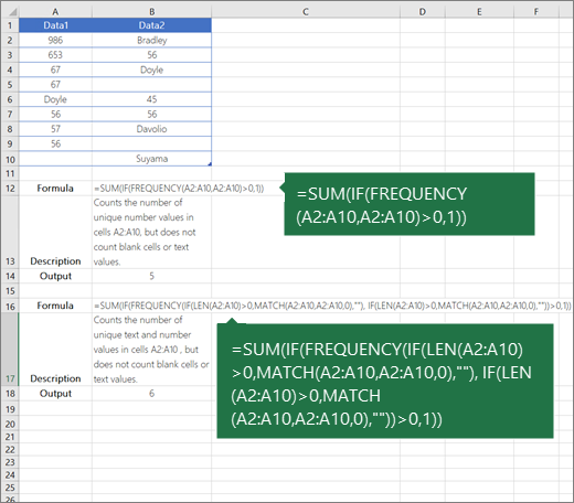
Let's say you want to find out how many unique values exist in a range that contains duplicate values. For example, if a column contains:

• The values 5, 6, 7, and 6, the result is three unique values — 5 , 6 and 7.

• The values "Bradley", "Doyle", "Doyle", "Doyle", the result is two unique values — "Bradley" and "Doyle".

There are several ways to count unique values among duplicates.

You can use the Advanced Filter dialog box to extract the unique values from a column of data and paste them to a new location. Then you can use the ROWS function to count the number of items in the new range.

1. Select the range of cells, or make sure the active cell is in a table.

   Make sure the range of cells has a column heading.

2. On the Data tab, in the Sort & Filter group, click Advanced.

   The Advanced Filter dialog box appears.

3. Click Copy to another location.

4. In the Copy to box, enter a cell reference.

   Alternatively, click Collapse Dialog to temporarily hide the dialog box, select a cell on the worksheet, and then press Expand Dialog .

5. Select the Unique records only check box, and click OK.

   The unique values from the selected range are copied to the new location beginning with the cell you specified in the Copy to box.

6. In the blank cell below the last cell in the range, enter the ROWS function. Use the range of unique values that you just copied as the argument, excluding the column heading. For example, if the range of unique values is B2:B45, you enter =ROWS(B2:B45).

Use a combination of the IF, SUM, FREQUENCY, MATCH, and LEN functions to do this task:

• Assign a value of 1 to each true condition by using the IF function.

• Add the total by using the SUM function.

• Count the number of unique values by using the FREQUENCY function. The FREQUENCY function ignores text and zero values. For the first occurrence of a specific value, this function returns a number equal to the number of occurrences of that value. For each occurrence of that same value after the first, this function returns a zero.

• Return the position of a text value in a range by using the MATCH function. This value returned is then used as an argument to the FREQUENCY function so that the corresponding text values can be evaluated.

• Find blank cells by using the LEN function. Blank cells have a length of 0.

Notes: 

• The formulas in this example must be entered as array formulas. If you have a current version of Microsoft 365, then you can simply enter the formula in the top-left-cell of the output range, then press ENTER to confirm the formula as a dynamic array formula. Otherwise, the formula must be entered as a legacy array formula by first selecting the output range, entering the formula in the top-left-cell of the output range, and then pressing CTRL+SHIFT+ENTER to confirm it. Excel inserts curly brackets at the beginning and end of the formula for you. For more information on array formulas, see Guidelines and examples of array formulas.

• To see a function evaluated step by step, select the cell containing the formula, and then on the Formulas tab, in the Formula Auditing group, click Evaluate Formula.

• The FREQUENCY function calculates how often values occur within a range of values, and then returns a vertical array of numbers. For example, use FREQUENCY to count the number of test scores that fall within ranges of scores. Because this function returns an array, it must be entered as an array formula.

• The MATCH function searches for a specified item in a range of cells, and then returns the relative position of that item in the range. For example, if the range A1:A3 contains the values 5, 25, and 38, the formula =MATCH(25,A1:A3,0) returns the number 2, because 25 is the second item in the range.

• The LEN function returns the number of characters in a text string.

• The SUM function adds all the numbers that you specify as arguments. Each argument can be a range, a cell reference, an array, a constant, a formula, or the result from another function. For example, SUM(A1:A5) adds all the numbers that are contained in cells A1 through A5.

• The IF function returns one value if a condition you specify evaluates to TRUE, and another value if that condition evaluates to FALSE.

Need more help?

You can always ask an expert in the Excel Tech Community or get support in the Answers community.

See Also

Filter for unique values or remove duplicate values