Add a watermark in Excel

Microsoft Excel doesn't come with a built-in watermark feature. However, there are a couple of ways that you can simulate the look of a watermark. In this topic we'll discuss how to create watermarks with images, like a company logo, and using an image as a worksheet background.

Can I insert a text watermark?

Excel does not support creation of text watermarks. Excel watermarks also do not support processes such as pasting in a block of text from Microsoft Word as a text watermark. You create the text you want for your watermark in a custom graphic in a standard picture file format such as .PNG, .JPG or .BMP, and import it into the Excel worksheet header. You can then use this picture as a watermark as many times as you want in your Excel worksheets.

1. Use your preferred graphics program, such as Microsoft Paint, to create the picture file with the text you want to use as your watermark.

2. In Excel, click Insert > Header & Footer. Excel changes to Page Layout View.

   

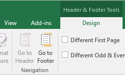
3. The Design tab appears under Header & Footer Tools.

   

4. The header appears directly above Row 1 of the worksheet, in three sections.

   

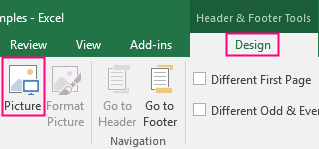
5. Click inside the left, center or right section for the header. In the Design ribbon, click Picture.

   

6. In the dialog box, click Browse. Browse to the picture you want to use, and double-click it. In the header, you'll see &[Picture]. This means there's a picture in the header.

   

7. Press the Tab key, or click anywhere outside the header. The company logo watermark appears in the currently displayed worksheet. When you create data on a new page in the same worksheet, the watermark appears on the new page.

   

   Notes: 

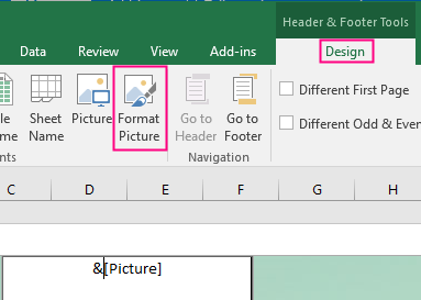
   • You may resize the watermark after you import it into Excel. In Page Layout mode, click the cursor in front of the "&" in &[Picture]. In the Design ribbon, click Format Picture. Use the Size tab to change the size of the watermark image on the worksheet. For other watermark settings, see the section Editing graphics properties for watermarks.

   • You'll see the watermark only when you're in Page Layout view or in Print Preview. The watermark also appears only on the current worksheet. You add a watermark to each worksheet in a workbook.

Insert a DRAFT watermark

When you share printouts of a worksheet and want people to know it's not the final copy, you can add the word "DRAFT" to the background on all the printed pages of your worksheet.

Note: You'll see the watermark only when you're in Page Layout view or in Print Preview. The watermark also appears only on the current worksheet. You add a watermark to each worksheet in a workbook.

1. Right-click this link (DRAFT), click Save picture as or Save target as..., and save the file to your computer. You can use this sample image for your watermark. )

2. In Excel, click Insert > Header & Footer. Excel changes to Page Layout View.

   

3. The Design tab appears under Header & Footer Tools.

   

4. The header appears directly above Row 1 of the worksheet, in three sections.

   

5. Click inside the left, center or right section for the header. In the Design ribbon, click Picture.

   

6. In the dialog box, click Browse. Browse to the picture you want to use, and double-click it. In the header, you'll see &[Picture]. This means there's a picture in the header.

   

7. Press the Tab key, or click anywhere outside the header. The new "DRAFT" watermark appears in the currently displayed worksheet. When you create data on a new page in the same worksheet, the watermark appears on the new page. The watermark does not appear in other worksheets in the same workbook. Each worksheet requires its own watermark.

   

   Note: You may resize the watermark after you import it into Excel. In Page Layout mode, click the cursor in front of the "&" in &[Picture]. In the Design ribbon, click Format Picture. Use the Size tab to change the size of the watermark image on the worksheet. For other watermark settings, see the section Editing graphics properties for watermarks.

Insert a Company Logo as a Watermark

When you want worksheet printouts to reflect your company brand, you can add a company logo graphic as a watermark on all the printed pages of your worksheet.

Note: You'll see the watermark only when you're in Page Layout view or in Print Preview. The watermark also appears only on the current worksheet. You add a watermark to each worksheet in a workbook.

1. In Excel, click Insert > Header & Footer. Excel changes to Page Layout View.

   

2. The Design tab appears under Header & Footer Tools.

   

3. The header appears directly above Row 1 of the worksheet, in three sections.

   

4. Click inside the left, center or right section for the header. In the Design ribbon, click Picture.

   

5. In the dialog box, click Browse. Browse to the picture you want to use, and double-click it. In the header, you'll see &[Picture]. This means there's a picture in the header.

   

6. Press the Tab key, or click anywhere outside the header. The company logo watermark appears in the currently displayed worksheet. When you create data on a new page in the same worksheet, the watermark appears on the new page.

   

   Note: You may resize the watermark after you import it into Excel. In Page Layout mode, click the cursor in front of the "&" in &[Picture]. In the Design ribbon, click Format Picture. Use the Size tab to change the size of the watermark image on the worksheet. For other watermark settings, see the section Editing graphics properties for watermarks.

Insert a CONFIDENTIAL Watermark

When you want people to know that your worksheet contains sensitive information that shouldn't be shared, add the word "CONFIDENTIAL" as a watermark on all the printed pages of your worksheet.

Note: You'll see the watermark only when you're in Page Layout view or in Print Preview. The watermark also appears only on the current worksheet. You add a watermark to each worksheet in a workbook.

1. Right-click this link (CONFIDENTIAL), click Save picture as or Save target as... , and save the file to your computer. This is the image you'll use for your watermark.

2. In Excel, click Insert > Header & Footer. Excel changes to Page Layout View.

   

3. The Design tab appears under Header & Footer Tools.

   

4. The header appears directly above Row 1 of the worksheet, in three sections.

   

5. Click inside the left, center or right section for the header. In the Design ribbon, click Picture.

   

6. In the dialog box, click Browse. Browse to the picture you want to use, and double-click it. In the header, you'll see &[Picture]. This means there's a picture in the header.

   

7. Press the Tab key, or click anywhere outside the header. The new "CONFIDENTIAL" watermark appears in the currently displayed worksheet. When you create data on a new page in the same worksheet, the watermark appears on the new page.

   

   Note: You may resize the watermark after you import it into Excel. In Page Layout mode, click the cursor in front of the "&" in &[Picture]. In the Design ribbon, click Format Picture. Use the Size tab to change the size of the watermark image on the worksheet. For other watermark settings, see the section Editing graphics properties for watermarks.

Insert a Background for your Worksheet

You can quickly experiment with backgrounds for your Excel worksheet. Unlike watermarks, backgrounds are viewable in Normal View in your worksheet, and are invisible in Page Layout mode.

1. Click Page Layout > Background.

2. In the dialog box, click Browse.

3. In the file requester, select the file you want to use and click Open.

   The image is automatically tiled on the background of the worksheet. Using this feature, the background is not inserted into the header section of the worksheet, which you do for a watermark.

   Notes: 

   • The background appears only on the current worksheet. If you want to use a watermark in the same worksheet as the background, the watermark appears over the background in your worksheet. Both the background and the watermark are visible (unless the watermark is the same size as the background image).

   • If the results of the background aren't what you want, click Page Layout > Remove Background.

Editing graphics properties for watermarks

You can change some basic graphics settings for watermarks, consisting of vertical centering for the watermark on the page, setting brightness and contrast, and sizing or scaling the watermark on the worksheet page. None of these settings apply to background graphics.

To define graphic properties for watermarks and backgrounds:

Centering the watermark

1. In Excel, click Insert > Header & Footer. Excel changes to Page Layout View.

   

2. The Design tab appears under Header & Footer Tools.

   

3. The header appears directly above Row 1 of the worksheet, in three sections. The watermark appears on the worksheet.

   

4. To center the watermark between the top and bottom of the page, select the header and make sure the cursor is in front of the "&" in &[Picture]. Then press Enter as many times as it takes to vertically align it the way you want. No adjustments are possible from left to right.

   

Setting brightness and contrast for the watermark

1. In Page Layout view, select the header and make sure the cursor is in front of the "&" in &[Picture].

2. Under Header & Footer Tools, click the Design tab > Format Picture.

   

3. On the Picture tab, under Image control, choose Washout in the Color box—this sets the Brightness level to 85% and Contrast to 15%. You can adjust brightness and contrast to suit your taste. To keep the picture's optimal balance, make sure the two levels add up to 100%; for example, 80% and 20% or 67% and 33%.

4. Under Header & Footer Tools, click the Design tab > Format Picture.

Sizing or scaling the watermark

1. Select the header and make sure the cursor is in front of the "&" in &[Picture].

   

2. Under Header & Footer Tools, click the Design tab > Format Picture.

   

3. On the Size tab, you can change the size of the picture by changing values in the Height and Width boxes. You can check or uncheck the Lock aspect ratio and Relative to original picture size boxes to control scaling.

Note: You'll see the watermark in Excel only when you're in Page Layout view or Print Preview. The watermark also appears only on the current worksheet. You add a watermark to each worksheet in a workbook.

Need more help?

You can always ask an expert in the Excel Tech Community, get support in the Answers community, or suggest a new feature or improvement on Excel User Voice.