Unpivot columns (Power Query)
Note: Power Query is known as Get & Transform in Excel 2016. Information provided here applies to both. To learn more, see Get & Transform in Excel 2016.
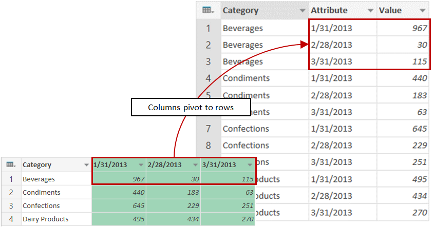
In Power Query, you can transform selected columns into attribute-value pairs where columns become rows. You use Power Query's Query Editor to unpivot columns.
Note: For a quick video on how to display Query Editor, see the end of this article.

First, select one or more columns in Query Editor. You can unpivot columns by using the Query Editor ribbon button, or by using a context menu.

Unpivot columns using the Query Editor ribbon:
-
In the Query Editor ribbon, click Unpivot Columns.
Unpivot columns using the Query Editor context menu:
-
Right-click the selected columns, and select Unpivot Columns.
Unpivot Columns creates an Attribute column for each selected column heading and a Value column for each selected column cell value. The attribute-value pair columns are inserted after the last column. In the example above, each date column becomes a row with an Attribute column containing the date value and a Value column containing the date column value. If you add an additional date column to the original source table, Power Query adds an additional row to the Unpivot table.

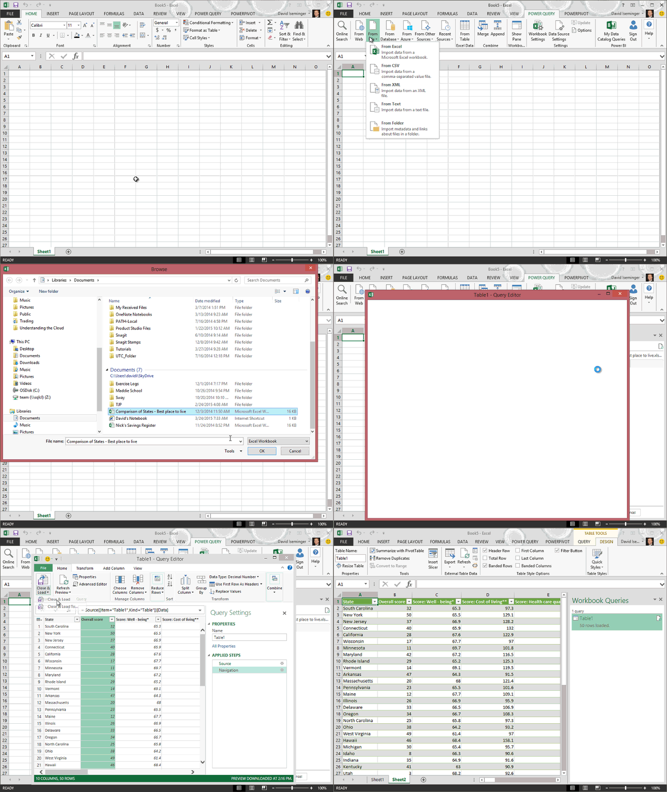
Note: The Query Editor only appears when you load, edit, or create a new query using Power Query. The following video shows the Query Editor window appearing after editing a query from an Excel workbook. To view the Query Editor without loading or editing an existing workbook query, from the Get External Data section in the Power Query ribbon tab, select From Other Sources > Blank Query. The following video shows one way to display the Query Editor.

No comments:
Post a Comment